Data discovery
Results: 162 items found

Air temperature - Venosta Valley
Daily averaged air temperature maps [C] maps for the Venosta Valley (South Tyrol,Italy) produced with the GEOtop hydrological model.
STAC
View
Sept. 2, 2019, 2 a.m.
 Aug. 2, 2020, 2 a.m.
Aug. 2, 2020, 2 a.m.
BoscoFontana
This collection is based on Sentinel-2 level 2A dataset acquired from both Sentinel-2 A and B satellites.
It covers a temporal range of 01-02-2021 to 30-09-2023, for every site all Sentinel scenes covering the area are included.
The collection includes all bands at a resolution of 10 meters. The bands are listed below.
B02
B03
B04
B05
B06
B07
B08
B8A
B09
B11
B12
SCL
The Level-2A data includes a Scene Classification, the algorithm allows the detection of clouds, snow and cloud shadows and generation of a classification map.
Cloud screening is applied to the data in order to retrieve accurate atmospheric and surface parameters during the atmospheric correction step.
The L2A SCL map can also be a valuable input for further processing steps or data analysis.
The collection covers all sites of the Hyperecos project. The following sites are included with the spatial extent mentioned.
Cireco {'west': 12.870775000000037, 'east': 13.103782000000024, 'south': 41.22186599400004, 'north': 41.41504699400008}
Orbetello {'west': 11.181888751927033,'east': 11.455397318265538, 'south': 42.372996996314896, 'north': 42.50311599528868}
Sciliar - Catinaccio {'west': 11.506713000000047, 'east': 11.667129000000045, 'south': 46.440615996000076, 'north': 46.54040999600005}
Castel Porziano {'west': 12.345466114000033, 'east': 12.451677663000055, 'south': 41.65575504100008, 'north': 41.78393419900004}
Monte Bondone {'west': 11.027602448000039, 'east': 11.044658587000072, 'south': 45.98801759300005, 'north': 46.01382867600006}
Bosco Fontana {'west': 10.73031770800003, 'east': 10.757708439000055, 'south': 45.192834764000054, 'north': 45.20899297600005}
Hunsrück-Hochwald {"west": 6.98720747225448, "east": 7.28904390300005, "north": 49.7943764377934, "south": 49.60530142600001}
STAC
View
May 1, 2021, 2 a.m.
Sept. 28, 2023, 2 a.m.
Sept. 28, 2023, 2 a.m.
CastelPorziano
This collection is based on Sentinel-2 level 2A dataset acquired from both Sentinel-2 A and B satellites.
It covers a temporal range of 01-02-2021 to 30-09-2023, for every site all Sentinel scenes covering the area are included.
The collection includes all bands at a resolution of 10 meters. The bands are listed below.
B02
B03
B04
B05
B06
B07
B08
B8A
B09
B11
B12
SCL
The Level-2A data includes a Scene Classification, the algorithm allows the detection of clouds, snow and cloud shadows and generation of a classification map.
Cloud screening is applied to the data in order to retrieve accurate atmospheric and surface parameters during the atmospheric correction step.
The L2A SCL map can also be a valuable input for further processing steps or data analysis.
The collection covers all sites of the Hyperecos project. The following sites are included with the spatial extent mentioned.
Cireco {'west': 12.870775000000037, 'east': 13.103782000000024, 'south': 41.22186599400004, 'north': 41.41504699400008}
Orbetello {'west': 11.181888751927033,'east': 11.455397318265538, 'south': 42.372996996314896, 'north': 42.50311599528868}
Sciliar - Catinaccio {'west': 11.506713000000047, 'east': 11.667129000000045, 'south': 46.440615996000076, 'north': 46.54040999600005}
Castel Porziano {'west': 12.345466114000033, 'east': 12.451677663000055, 'south': 41.65575504100008, 'north': 41.78393419900004}
Monte Bondone {'west': 11.027602448000039, 'east': 11.044658587000072, 'south': 45.98801759300005, 'north': 46.01382867600006}
Bosco Fontana {'west': 10.73031770800003, 'east': 10.757708439000055, 'south': 45.192834764000054, 'north': 45.20899297600005}
Hunsrück-Hochwald {"west": 6.98720747225448, "east": 7.28904390300005, "north": 49.7943764377934, "south": 49.60530142600001}
STAC
View
May 5, 2021, 2 a.m.
Sept. 27, 2023, 2 a.m.
Sept. 27, 2023, 2 a.m.
CERRA-Land sub-daily regional reanalysis data for the European Alps for 2001
The Copernicus European Regional ReAnalysis Land (CERRA-Land) dataset provides spatially and temporally consistent historical reconstructions of surface and soil variables at the same horizontal resolution as the CERRA high-resolution reanalysis.
STAC
View
Jan. 1, 2001, 1 a.m.
Dec. 31, 2001, 1 a.m.
Dec. 31, 2001, 1 a.m.
CERRA-Land sub-daily regional reanalysis orography data for the European Alps
The Copernicus European Regional ReAnalysis Land (CERRA-Land) Orography dataset provides spatially and temporally consistent historical reconstructions of orography at the same horizontal resolution as the CERRA high-resolution reanalysis.
STAC
View
Jan. 1, 2020, 1 a.m.
Jan. 1, 2020, 1 a.m.
Jan. 1, 2020, 1 a.m.
CERRA sub-daily regional reanalysis data for the European Alps on single levels
The Copernicus European Regional ReAnalysis (CERRA) datasets provide spatially and temporally consistent historical reconstructions of meteorological variables in the atmosphere and at the surface.
STAC
View
Jan. 1, 2001, 1 a.m.
Dec. 31, 2001, 1 a.m.
Dec. 31, 2001, 1 a.m.
CERRA sub-daily regional reanalysis data for the European Alps on single levels
The Copernicus European Regional ReAnalysis (CERRA) datasets provide spatially and temporally consistent historical reconstructions of meteorological variables in the atmosphere and at the surface.
STAC
View
Jan. 1, 2001, 1 a.m.
Dec. 31, 2001, 1 a.m.
Dec. 31, 2001, 1 a.m.
Cleaned EPC for residential building of Lombardia Region - Cened1.2+
Cleaned EPC for residential building of Lombardia Region - Cened1.2+
Other
View
Copernicus Land Monitoring Service - EU-DEM
EU-DEM is a digital surface model (DSM) of EEA member and cooperating countries representing the first surface as illuminated by the sensors. It is a hybrid product based on SRTM and ASTER GDEM data fused by a weighted averaging approach.
STAC
View
Jan. 1, 2019, 1 a.m.
None
None
Copernicus Land Monitoring Service - Surface Soil Moisture indexed with Kerchunk around the original netCDFs.
Copernicus Land Monitoring Service - Surface Soil Moisture 2014-present (raster 1 km), Europe, daily – version 1
STAC
View
Oct. 3, 2014, 2 a.m.
Aug. 17, 2024, 2 a.m.
Aug. 17, 2024, 2 a.m.
Copernicus_Senwise_CHIME-like_BE
The input CHIME-like imagery dataset is produced based on EnMAP L2A and PRISMA L2D hyperspectral product respectivelly downloaded from EnMAP catalog (https://eoweb.dlr.de/egp/main) and from ASI PRISMA catalog (http://prisma.asi.it/js-cat-client-prisma-src) . The CHIME-like imagery aims to simulate the future CHIME sensor at Level 2 (Bottom-of-Atmosphere BOA reflectance) and consists of 192 spectral bands from 415 - 2450 nm with a band width of around 12 nm.
STAC
View
April 8, 2020, 12:42 p.m.
Sept. 19, 2024, 1:14 p.m.
Sept. 19, 2024, 1:14 p.m.
Copernicus_Senwise_CHIME-like_FR
The input CHIME-like imagery dataset is produced based on EnMAP L2A and PRISMA L2D hyperspectral product respectivelly downloaded from EnMAP catalog (https://eoweb.dlr.de/egp/main) and from ASI PRISMA catalog (http://prisma.asi.it/js-cat-client-prisma-src) . The CHIME-like imagery aims to simulate the future CHIME sensor at Level 2 (Bottom-of-Atmosphere BOA reflectance) and consists of 193 spectral bands from 415 - 2450 nm with a band width of around 12 nm.
STAC
View
Jan. 6, 2020, 11:41 a.m.
July 28, 2025, 12:41 p.m.
July 28, 2025, 12:41 p.m.
Copernicus Senwise RoseL-like imagery, Aix-en-Provence_Pennes-Mirabeau, FR 3, 2025
The input RoseL-like imagery dataset is a copy of SAOCOM-1B SAR Stripmap dual pol (VH-VV) data collection downloaded from saocom.asi.it. Data are in the Single Look Complex (SLC - Level-1A) format suitable for InSAR/PolSAR processing. Data cover the Aix-en-Provence region, in South of France, including the Pennes-Mirabeau area, where wildfires happened in Summer 2025. Coordinates are [5.23, 43.71], [5.85, 42.93]. Data are acquired in descending (DSC) orbit and are given here in the SAR acquisition geometry (slant range, azimuth coordinates). Both extent and numbers of rows and columns vary a bit from one image to the other: values given here correspond to the 1st image of the collection. One geoprojected (.tif) image out of the collection is provided for information only, for allowing to locate the relevant area.
STAC
View
June 25, 2025, 7:40 p.m.
Sept. 29, 2025, 7:41 p.m.
Sept. 29, 2025, 7:41 p.m.
Copernicus Senwise RoseL-like imagery, GrandLeez, BE 1, 2022
The input RoseL-like imagery dataset is a copy of SAOCOM-1A L-band SAR Stripmap dual pol (VH-VV) data collection over a sub-region of Wallon Region, Belgium, downloaded from saocom.asi.it. Data are in the Single Look Complex (SLC - Level-1A) format suitable for InSAR/PolSAR processing. Data are acquired in ascending (ASC) orbit and are given/provided here in the SAR acquisition geometry (slant range, azimuth coordinates). Both extent and numbers of rows and columns vary a bit from one image to the other: values given here correspond to the 1st image of the collection. A geoprojected (.tif) image out of the collection is provided for information only, for allowing to locate the relevant area.
STAC
View
July 30, 2022, 7:18 a.m.
Dec. 22, 2022, 12:59 a.m.
Dec. 22, 2022, 12:59 a.m.
Copernicus Senwise RoseL-like imagery, Martigues, FR 1, 2025
The input RoseL-like imagery dataset is a copy of SAOCOM-1A SAR Stripmap dual pol (VH-VV) data collection downloaded from saocom.asi.it. Data are in the Single Look Complex (SLC - Level-1A) format suitable for InSAR/PolSAR processing. Data cover the Martigues area, South of France, where a wildfire happened in Summer 2025. Coordinates are [4.43, 43.44], [5.36, 42.92]. Data are acquired in ascending (ASC) orbit and are given here in the SAR acquisition geometry (slant range, azimuth coordinates). Both extent and numbers of rows and columns vary a bit from one image to the other: values given here correspond to the 1st image of the collection. One geoprojected (.tif) image out of the collection is provided for information only, for allowing to locate the relevant area.
STAC
View
June 26, 2025, 7:28 a.m.
Sept. 30, 2025, 7:29 a.m.
Sept. 30, 2025, 7:29 a.m.
Copernicus Senwise RoseL-like imagery - Mazia Matsch catchment, South Tyrol, IT, 2023
The input RoseL-like imagery dataset is a copy of SAOCOM-1A SAR Stripmap dual pol (VH-VV) data collection downloaded from saocom.asi.it and covering the Glorenza-Merano region, including the Mazia-Matsch catchment, in South-Tyrol, Italy. Coordinates are [10.29, 46.96], [11.27, 46.38]. Data are in the Single Look Complex (SLC - Level-1A) format suitable for InSAR/PolSAR processing. Data are acquired in ascending (ASC) orbit and are given here in the SAR acquisition geometry (slant range, azimuth coordinates). Both extent and numbers of rows and columns vary a bit from one image to the other: values given here correspond to the 1st image of the collection. One geoprojected (.tif) image out of the collection is provided for information only, for allowing to locate the relevant area.
STAC
View
Aug. 1, 2023, 6:57 a.m.
Dec. 7, 2023, 5:59 a.m.
Dec. 7, 2023, 5:59 a.m.
Copernicus Senwise RoseL-like imagery - Mazia Matsch catchment, South Tyrol, IT, 2024
The input RoseL-like imagery dataset is a copy of SAOCOM-1A SAR Stripmap dual pol (VH-VV) data collection downloaded from saocom.asi.it and covering the Glorenza-Merano region, including the Mazia-Matsch catchment, in South-Tyrol, Italy. Coordinates are [10.33, 46.91], [11.33, 46.28]. Data are in the Single Look Complex (SLC - Level-1A) format suitable for InSAR/PolSAR processing. Data are acquired in ascending (ASC) orbit and are given here in the SAR acquisition geometry (slant range, azimuth coordinates). Both extent and numbers of rows and columns vary a bit from one image to the other: values given here correspond to the 1st image of the collection. One geoprojected (.tif) image out of the collection is provided for information only, for allowing to locate the relevant area.
STAC
View
Jan. 8, 2024, 5:57 a.m.
Dec. 25, 2024, 5:59 a.m.
Dec. 25, 2024, 5:59 a.m.
Copernicus Senwise RoseL-like imagery - Mazia Matsch catchment, South Tyrol, IT, 2025
The input RoseL-like imagery dataset is a copy of SAOCOM-1A SAR Stripmap dual pol (VH-VV) data collection downloaded from saocom.asi.it and covering the Glorenza-Merano region, including the Mazia-Matsch catchment, in South-Tyrol, Italy. Coordinates are [10.30, 46.92], [11.29, 46.34]. Data are in the Single Look Complex (SLC - Level-1A) format suitable for InSAR/PolSAR processing. Data are acquired in ascending (ASC) orbit and are given here in the SAR acquisition geometry (slant range, azimuth coordinates). Both extent and numbers of rows and columns vary a bit from one image to the other: values given here correspond to the 1st image of the collection. One geoprojected (.tif) image out of the collection is provided for information only, for allowing to locate the relevant area.
STAC
View
Jan. 26, 2025, 5:57 a.m.
Nov. 10, 2025, 5:59 a.m.
Nov. 10, 2025, 5:59 a.m.
Copernicus Senwise RoseL-like imagery, Vidauban, FR 2, 2024
The input RoseL-like imagery dataset is a copy of SAOCOM-1B SAR Stripmap dual pol (VH-VV) data collection downloaded from saocom.asi.it. Data are in the Single Look Complex (SLC - Level-1A) format suitable for InSAR/PolSAR processing. Coordinates are [5.95, 43.46], [6.90, 42.88]. Data cover the Vidauban area, South of France, where a wildfire happened in Summer 2024. Data are acquired in ascending (ASC) orbit and are given here in the SAR acquisition geometry (slant range, azimuth coordinates). Both extent and numbers of rows and columns vary a bit from one image to the other: values given here correspond to the 1st image of the collection. One geoprojected (.tif) image out of the collection is provided for information only, for allowing to locate the relevant area.
STAC
View
May 3, 2024, 7:19 a.m.
Sept. 24, 2024, 7:20 a.m.
Sept. 24, 2024, 7:20 a.m.
Copernicus Senwise RoseL-like imagery - Walloon Region - BE 1, 2025
The input RoseL-like imagery dataset is a copy of SAOCOM-1A SAR Stripmap dual pol (VH-VV) data collection over a sub-region of Wallon Region, Belgium, downloaded from saocom.asi.it. Coordinates are [4.51,51.04], [5.58,50.53]. Data are in the Single Look Complex (SLC - Level-1A) format suitable for InSAR/PolSAR processing. Data are acquired in ascending (ASC) orbit and are given here in the SAR acquisition geometry (slant range, azimuth coordinates). Both extent and numbers of rows and columns vary a bit from one image to the other: values given here correspond to the 1st image of the collection. One geoprojected (.tif) image out of the collection is provided for information only, for allowing to locate the relevant area.
STAC
View
Oct. 10, 2025, 7:18 a.m.
Nov. 11, 2025, 6:19 a.m.
Nov. 11, 2025, 6:19 a.m.
Copernicus Senwise RoseL-like imagery, Walloon Region, BE 3, 2025
The input RoseL-like imagery dataset is a copy of SAOCOM-1A SAR Stripmap dual pol (VH-VV) data collection over a sub-region of Wallon Region, Belgium, downloaded from saocom.asi.it. Coordinates are [4.02, 50.78], [4.73, 50.06]. Data are in the Single Look Complex (SLC - Level-1A) format suitable for InSAR/PolSAR processing. Data are acquired in descending (DSC) orbit and are given here in the SAR acquisition geometry (slant range, azimuth coordinates). Both extent and numbers of rows and columns vary a bit from one image to the other: values given here correspond to the 1st image of the collection. One geoprojected (.tif) image out of the collection is provided for information only, for allowing to locate the relevant area.
STAC
View
April 20, 2025, 7:54 p.m.
Nov. 14, 2025, 6:56 p.m.
Nov. 14, 2025, 6:56 p.m.
Copernicus Senwise RoseL-like imagery, Walloon Region, BE 4, 2025
The input RoseL-like imagery dataset is a copy of SAOCOM-1A SAR Stripmap dual pol (VH-VV) data collection over a sub-region of Wallon Region, Belgium, downloaded from saocom.asi.it. Coordinates are [5.36,50.20], [6.05,49.42]. Data are in the Single Look Complex (SLC - Level-1A) format suitable for InSAR/PolSAR processing. Data are acquired in descending (DSC) orbit and are given here in the SAR acquisition geometry (slant range, azimuth coordinates). Both extent and numbers of rows and columns vary a bit from one image to the other: values given here correspond to the 1st image of the collection. One geoprojected (.tif) image out of the collection is provided for information only, for allowing to locate the relevant area.
STAC
View
June 28, 2025, 7:48 p.m.
Nov. 19, 2025, 6:50 p.m.
Nov. 19, 2025, 6:50 p.m.
Copernicus Senwise RoseL-like imagery, Walloon Region, BE 5, 2025
The input RoseL-like imagery dataset is a copy of SAOCOM-1A L-band SAR Stripmap dual pol (VH-VV) data collection downloaded from saocom.asi.it, Acquisitions cover a sub-region of Wallon Region, Belgium, including the forest of Grand-Leez, for 2022. Coordinates are [4.52,51.00], [5.60,50.49]. Data are in the Single Look Complex (SLC - Level-1A) format suitable for InSAR/PolSAR processing. Data are acquired in ascending (ASC) orbit and are given/provided here in the SAR acquisition geometry (slant range, azimuth coordinates). Both extent and numbers of rows and columns vary a bit from one image to the other: values given here correspond to the 1st image of the collection. A geoprojected (.tif) image out of the collection is provided for information only, for allowing to locate the relevant area.
STAC
View
June 15, 2025, 7:50 p.m.
Nov. 22, 2025, 6:52 p.m.
Nov. 22, 2025, 6:52 p.m.
Copernicus Senwise RoseL-like imagery, Walloon Region, Tellin, BE 2, 2024
The input RoseL-like imagery dataset is a copy of SAOCOM-1A L-band SAR Stripmap dual pol (VH-VV) data collection downloaded from saocom.asi.it, Acquisitions cover a sub-region of Wallon Region, Belgium, including the forest of Grand-Leez, for 2022. Coordinates are [4.52,51.00], [5.60,50.49]. Data are in the Single Look Complex (SLC - Level-1A) format suitable for InSAR/PolSAR processing. Data are acquired in ascending (ASC) orbit and are given/provided here in the SAR acquisition geometry (slant range, azimuth coordinates). Both extent and numbers of rows and columns vary a bit from one image to the other: values given here correspond to the 1st image of the collection. A geoprojected (.tif) image out of the collection is provided for information only, for allowing to locate the relevant area.
STAC
View
March 29, 2024, 6:17 a.m.
Dec. 26, 2024, 6:19 a.m.
Dec. 26, 2024, 6:19 a.m.
CORINE Land Cover 2018 (CLC2018), Europe (Raster 100m)
The Corine Land Cover 2018 (CLC2018) dataset is one of the datasets produced within the CORINE Land Cover Program to capture land cover/ land use status for 2018. The Corine Land Cover (CLC) is an European programme, coordinated by the European Environment Agency (EEA), providing consistent information on land cover and land cover changes across Europe. CLC products are based on the photointerpretation of satellite images by the national teams of the participating countries - the EEA member or cooperating countries. The resulting national land cover inventories are further integrated into a seamless land cover map of Europe. The resulting European database is based on standard methodology and nomenclature with following base parameters: - 44 thematic classes in the hierarchical 3-level Corine nomenclature - minimum mapping unit (MMU) for status layers is 25 hectares - minimum width of linear elements is 100 metres - minimum mapping unit (MMU) for Land Cover Changes (LCC) for change layers is 5 hectares. It is provided as 100m raster data here
STAC
View
Jan. 1, 2018, 1 a.m.
Jan. 1, 2018, 1 a.m.
Jan. 1, 2018, 1 a.m.
Corine Land Cover (CLC) 2018
CLC2018 is one of the Corine Land Cover (CLC) datasets produced within the frame the Copernicus Land Monitoring Service referring to land cover / land use status of year 2018. CLC service has a long-time heritage (formerly known as "CORINE Land Cover Programme"), coordinated by the European Environment Agency (EEA). It provides consistent and thematically detailed information on land cover and land cover changes across Europe.
STAC
View
Jan. 1, 2017, 1 a.m.
Dec. 31, 2021, 1 a.m.
Dec. 31, 2021, 1 a.m.
Daily evaporation product Ebro basin
Daily evaporation data are produced from Two-Source Energy Balanced (TSEB) model driven by ESA Sentinel (both Sentinel-2 MSI and Sentinel-3 SLSTR) and ERA5 reanalysis data
STAC
View
Jan. 1, 2017, 1 a.m.
Dec. 31, 2021, 1 a.m.
Dec. 31, 2021, 1 a.m.
Daily evaporation product Herault basin
Daily evaporation data are produced from Two-Source Energy Balanced (TSEB) model driven by ESA Sentinel (both Sentinel-2 MSI and Sentinel-3 SLSTR) and ERA5 reanalysis data
STAC
View
Jan. 1, 2017, 1 a.m.
Dec. 31, 2021, 1 a.m.
Dec. 31, 2021, 1 a.m.
Daily evaporation product Medjerda basin
Daily evaporation data are produced from Two-Source Energy Balanced (TSEB) model driven by ESA Sentinel (both Sentinel-2 MSI and Sentinel-3 SLSTR) and ERA5 reanalysis data
STAC
View
Jan. 1, 2017, 1 a.m.
Dec. 31, 2021, 1 a.m.
Dec. 31, 2021, 1 a.m.
Daily evaporation product Po basin
Daily evaporation data are produced from Two-Source Energy Balanced (TSEB) model driven by ESA Sentinel (both Sentinel-2 MSI and Sentinel-3 SLSTR) and ERA5 reanalysis data
STAC
View
Jan. 1, 2017, 1 a.m.
Dec. 31, 2021, 1 a.m.
Dec. 31, 2021, 1 a.m.
Daily evapotranspiration product - 60m - 32TPS
Developed through the SENWISE project, this daily evapotranspiration (ET) demonstrates the type of ET products that could be generated from LSTM-like consolidated datasets, thereby supporting the assessment of their potential for agricultural and environmental applications. The dataset provides a consolidated, multi-temporal representation of daily ET, generated from the high-resolution LST products Land Surface Temperature Monitoring (LSTM) representative dataset product at 60m resolution developed within the project, together with ancillary structural, biophysical, and meteorological datasets. ET is provided at 60m resolution and is produced using the TSEB-PT model (Norman et al., 1995). Data collection covers the area of Sentinel-2 Tile: 32TPS (WGS84, EPSG4326: 10.2904840, 45.9334965, 11.7555849, 46.9461682). ET is provided in mm/day and stored with a scale factor of 0.01.
STAC
View
April 1, 2017, 2 a.m.
Nov. 1, 2025, 12:59 a.m.
Nov. 1, 2025, 12:59 a.m.
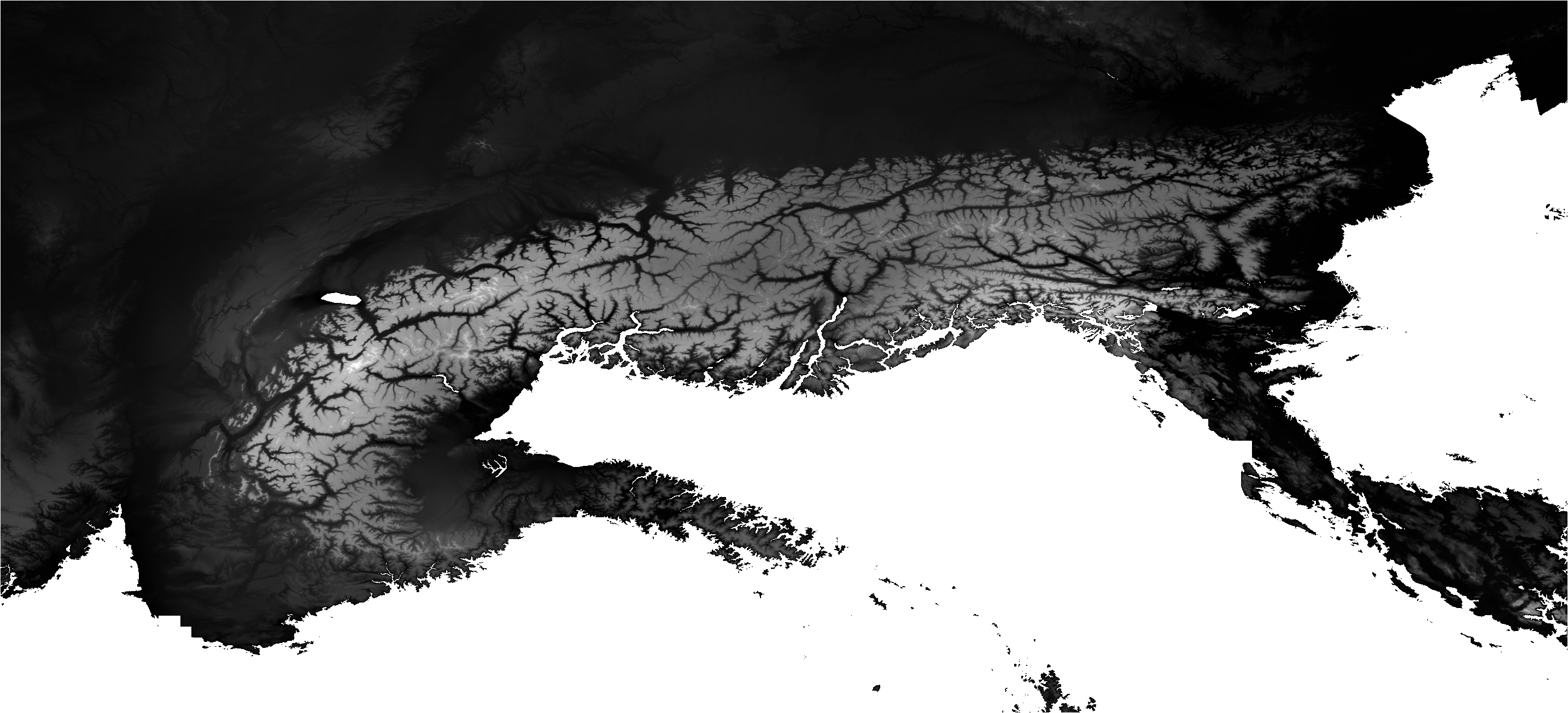
Daily Height of Snow for the European Alps
S3M-Alps is a 500-m reanalysis of Snow Water Equivalent and Height of Snow for the European Alps. The product is driven by ERA5-Land meteorological reanalysis downscaled to 500 m using the MicroMet statistical–dynamical method (Liston and Elder, 2006). Downscaled meteorological fields are used to force the physically-based S3M snow model (Avanzi et al., 2022).
STAC
View
Sept. 1, 1950, 1 a.m.
Dec. 31, 2025, 1 a.m.
Dec. 31, 2025, 1 a.m.

Daily precipitation product
Daily precipitation (P) data at 1 km spatial resolution - Data are obtained by downscaling CPC and GPM-LR data to 1 km spatial resolution using CHELSA climatology and merging them through a triple collocation technique on CPC GPM and ERA5
STAC
View
Jan. 1, 2000, 1 a.m.
Feb. 28, 2022, 1 a.m.
Feb. 28, 2022, 1 a.m.
Daily precipitation product - 1000m
Daily precipitation (P) data at 1 km spatial resolution - Data are obtained by downscaling CPC and GPM-LR data to 1 km spatial resolution using CHELSA climatology and merging them through a triple collocation technique on CPC GPM and ERA5
STAC
View
Jan. 1, 2000, 1 a.m.
Feb. 28, 2022, 1 a.m.
Feb. 28, 2022, 1 a.m.
Daily Snow Water Equivalent-1000m
A 1km experimental dataset for the Mediterranean terrestrial region of Snow Water Equivalent from the assimilation of Sentinel-1 C-SNOW data into the S3M model
STAC
View
Aug. 1, 2015, 2 a.m.
Dec. 31, 2021, 1 a.m.
Dec. 31, 2021, 1 a.m.
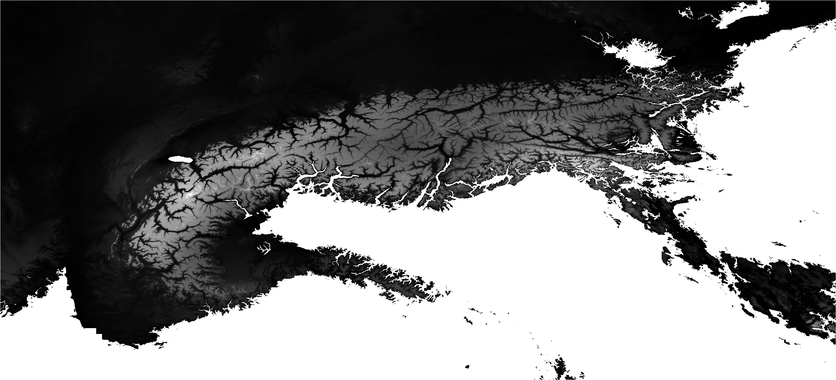
Daily Snow Water Equivalent for the European Alps
S3M-Alps is a 500-m reanalysis of Snow Water Equivalent for the European Alps. The product is driven by ERA5-Land meteorological reanalysis downscaled to 500 m using the MicroMet statistical–dynamical method (Liston and Elder, 2006). Downscaled meteorological fields are used to force the physically-based S3M snow model (Avanzi et al., 2022).
STAC
View
Sept. 1, 1950, 1 a.m.
Dec. 31, 2025, 1 a.m.
Dec. 31, 2025, 1 a.m.
Daily Surface Soil Moisture
A 1km experimental dataset for the Mediterranean terrestrial region of Soil Moisture,Land Surface Temperature and Vegetation Optical Depth from passive microwave data.
STAC
View
Jan. 1, 2017, 1 p.m.
Dec. 31, 2021, 1 p.m.
Dec. 31, 2021, 1 p.m.
Daily TWSC product-Ebro
A 1km experimental dataset for the four Mediterranean basins of daily TWSC data from GRACE monthly JPL mascon and a water budget model driven by GLEAM-1k SM2RAIN_GPM_CPC and HDMA model
STAC
View
Jan. 1, 2017, 1 a.m.
Dec. 31, 2021, 1 a.m.
Dec. 31, 2021, 1 a.m.
Daily TWSC product-Po
A 1km experimental dataset for the four Mediterranean basins of daily TWSC data from GRACE monthly JPL mascon and a water budget model driven by GLEAM-1k SM2RAIN_GPM_CPC and HDMA model
STAC
View
Jan. 1, 2017, 1 a.m.
Dec. 31, 2019, 1 a.m.
Dec. 31, 2019, 1 a.m.
Daytime land surface temperature product - 60m - 31TGJ
Developed through the SENWISE initiative, this Land Surface Temperature Monitoring (LSTM) representative dataset aims to support the preparation of the upcoming mission by emulating its expected data products. The dataset provides a consolidated, multi-temporal representation of daytime land surface temperature (LST), structured to be a proxy of the future LSTM data outputs. Data are provided at 60m resolution and are produced using Sentinel-3 LST product at 1km resolution through Kernel Driven Downscaling (KDD). Data collection covers the area of Sentinel 2 Tile: 32TGJ (WGS84, EPSG4326: 5.4627354, 43.2012113, 6.8757389, 44.2259751). LST is provided in Kelvin and stored with an offset of 150, a scale factor of 0.01.
STAC
View
April 1, 2017, 2 a.m.
Nov. 1, 2025, 12:59 a.m.
Nov. 1, 2025, 12:59 a.m.
Daytime land surface temperature product - 60m - 31UFR
Developed through the SENWISE initiative, this Land Surface Temperature Monitoring (LSTM) representative dataset aims to support the preparation of the upcoming mission by emulating its expected data products. The dataset provides a consolidated, multi-temporal representation of daytime land surface temperature (LST), structured to be a proxy of the future LSTM data outputs. Data are provided at 60m resolution and are produced using Sentinel-3 LST product at 1km resolution through Kernel Driven Downscaling (KDD). Data collection covers the area of Sentinel 2 Tile: 31UFR (WGS84, EPSG4326: 4.3826843, 49.5284182, 5.9593860, 50.5437391). LST is provided in Kelvin and stored with an offset of 150, a scale factor of 0.01.
STAC
View
April 1, 2017, 2 a.m.
Nov. 1, 2025, 12:59 a.m.
Nov. 1, 2025, 12:59 a.m.
Daytime land surface temperature product - 60m - 32TPS
Developed through the SENWISE initiative, this Land Surface Temperature Monitoring (LSTM) representative dataset aims to support the preparation of the upcoming mission by emulating its expected data products. The dataset provides a consolidated, multi-temporal representation of daytime land surface temperature (LST), structured to be a proxy of the future LSTM data outputs. Data are provided at 60m resolution and are produced using Sentinel-3 LST product at 1km resolution through Kernel Driven Downscaling (KDD). Data collection covers the area of Sentinel 2 Tile: 32TPS (WGS84, EPSG4326: 10.2904840, 45.9334965, 11.7555849, 46.9461682). LST is provided in Kelvin and stored with an offset of 150, a scale factor of 0.01.
STAC
View
April 1, 2017, 2 a.m.
Nov. 1, 2025, 12:59 a.m.
Nov. 1, 2025, 12:59 a.m.
E_GLEAM_1km_2015-2021_D0_SSpain
Daily land evaporation (mm/day) estimated from a fully satellite driven evaporation model GLEAM v3. E is calculated as a sum of interception loss, transpiration and bare soil evaporation. The latter two are based on a Priestley and Taylor equation constrained by soil and vegetation water content.
STAC
View
Jan. 1, 2015, 1 a.m.
Dec. 31, 2021, 1 a.m.
Dec. 31, 2021, 1 a.m.
E_GLEAM_1km_2015-2021_D10_SardiniaCorsica
Daily land evaporation (mm/day) estimated from a fully satellite driven evaporation model GLEAM v3. E is calculated as a sum of interception loss, transpiration and bare soil evaporation. The latter two are based on a Priestley and Taylor equation constrained by soil and vegetation water content.
STAC
View
Jan. 1, 2015, 1 a.m.
Dec. 31, 2021, 1 a.m.
Dec. 31, 2021, 1 a.m.
E_GLEAM_1km_2015-2021_D11_Istria
Daily land evaporation (mm/day) estimated from a fully satellite driven evaporation model GLEAM v3. E is calculated as a sum of interception loss, transpiration and bare soil evaporation. The latter two are based on a Priestley and Taylor equation constrained by soil and vegetation water content.
STAC
View
Jan. 1, 2015, 1 a.m.
Dec. 31, 2021, 1 a.m.
Dec. 31, 2021, 1 a.m.
E_GLEAM_1km_2015-2021_D12_Dalmatia
Daily land evaporation (mm/day) estimated from a fully satellite driven evaporation model GLEAM v3. E is calculated as a sum of interception loss, transpiration and bare soil evaporation. The latter two are based on a Priestley and Taylor equation constrained by soil and vegetation water content.
STAC
View
Jan. 1, 2015, 1 a.m.
Dec. 31, 2021, 1 a.m.
Dec. 31, 2021, 1 a.m.
E_GLEAM_1km_2015-2021_D13_Epirus
Daily land evaporation (mm/day) estimated from a fully satellite driven evaporation model GLEAM v3. E is calculated as a sum of interception loss, transpiration and bare soil evaporation. The latter two are based on a Priestley and Taylor equation constrained by soil and vegetation water content.
STAC
View
Jan. 1, 2015, 1 a.m.
Dec. 31, 2021, 1 a.m.
Dec. 31, 2021, 1 a.m.
E_GLEAM_1km_2015-2021_D14_Bulgaria
Daily land evaporation (mm/day) estimated from a fully satellite driven evaporation model GLEAM v3. E is calculated as a sum of interception loss, transpiration and bare soil evaporation. The latter two are based on a Priestley and Taylor equation constrained by soil and vegetation water content.
STAC
View
Jan. 1, 2015, 1 a.m.
Dec. 31, 2021, 1 a.m.
Dec. 31, 2021, 1 a.m.
E_GLEAM_1km_2015-2021_D15_Greece
Daily land evaporation (mm/day) estimated from a fully satellite driven evaporation model GLEAM v3. E is calculated as a sum of interception loss, transpiration and bare soil evaporation. The latter two are based on a Priestley and Taylor equation constrained by soil and vegetation water content.
STAC
View
Jan. 1, 2015, 1 a.m.
Dec. 31, 2021, 1 a.m.
Dec. 31, 2021, 1 a.m.
E_GLEAM_1km_2015-2021_D16_SWTurkey
Daily land evaporation (mm/day) estimated from a fully satellite driven evaporation model GLEAM v3. E is calculated as a sum of interception loss, transpiration and bare soil evaporation. The latter two are based on a Priestley and Taylor equation constrained by soil and vegetation water content.
STAC
View
Jan. 1, 2015, 1 a.m.
Dec. 31, 2021, 1 a.m.
Dec. 31, 2021, 1 a.m.
E_GLEAM_1km_2015-2021_D17_Cyprus
Daily land evaporation (mm/day) estimated from a fully satellite driven evaporation model GLEAM v3. E is calculated as a sum of interception loss, transpiration and bare soil evaporation. The latter two are based on a Priestley and Taylor equation constrained by soil and vegetation water content.
STAC
View
Jan. 1, 2015, 1 a.m.
Dec. 31, 2021, 1 a.m.
Dec. 31, 2021, 1 a.m.
E_GLEAM_1km_2015-2021_D18_Antioch
Daily land evaporation (mm/day) estimated from a fully satellite driven evaporation model GLEAM v3. E is calculated as a sum of interception loss, transpiration and bare soil evaporation. The latter two are based on a Priestley and Taylor equation constrained by soil and vegetation water content.
STAC
View
Jan. 1, 2015, 1 a.m.
Dec. 31, 2021, 1 a.m.
Dec. 31, 2021, 1 a.m.
E_GLEAM_1km_2015-2021_D19_Cairo
Daily land evaporation (mm/day) estimated from a fully satellite driven evaporation model GLEAM v3. E is calculated as a sum of interception loss, transpiration and bare soil evaporation. The latter two are based on a Priestley and Taylor equation constrained by soil and vegetation water content.
STAC
View
Jan. 1, 2015, 1 a.m.
Dec. 31, 2021, 1 a.m.
Dec. 31, 2021, 1 a.m.
E_GLEAM_1km_2015-2021_D1_ESpain
Daily land evaporation (mm/day) estimated from a fully satellite driven evaporation model GLEAM v3. E is calculated as a sum of interception loss, transpiration and bare soil evaporation. The latter two are based on a Priestley and Taylor equation constrained by soil and vegetation water content.
STAC
View
Jan. 1, 2015, 1 a.m.
Dec. 31, 2021, 1 a.m.
Dec. 31, 2021, 1 a.m.
E_GLEAM_1km_2015-2021_D20_WEgypt
Daily land evaporation (mm/day) estimated from a fully satellite driven evaporation model GLEAM v3. E is calculated as a sum of interception loss, transpiration and bare soil evaporation. The latter two are based on a Priestley and Taylor equation constrained by soil and vegetation water content.
STAC
View
Jan. 1, 2015, 1 a.m.
Dec. 31, 2021, 1 a.m.
Dec. 31, 2021, 1 a.m.
E_GLEAM_1km_2015-2021_D21_Cyrenaica
Daily land evaporation (mm/day) estimated from a fully satellite driven evaporation model GLEAM v3. E is calculated as a sum of interception loss, transpiration and bare soil evaporation. The latter two are based on a Priestley and Taylor equation constrained by soil and vegetation water content.
STAC
View
Jan. 1, 2015, 1 a.m.
Dec. 31, 2021, 1 a.m.
Dec. 31, 2021, 1 a.m.
E_GLEAM_1km_2015-2021_D22_ELibya
Daily land evaporation (mm/day) estimated from a fully satellite driven evaporation model GLEAM v3. E is calculated as a sum of interception loss, transpiration and bare soil evaporation. The latter two are based on a Priestley and Taylor equation constrained by soil and vegetation water content.
STAC
View
Jan. 1, 2015, 1 a.m.
Dec. 31, 2021, 1 a.m.
Dec. 31, 2021, 1 a.m.
E_GLEAM_1km_2015-2021_D23_WLibya
Daily land evaporation (mm/day) estimated from a fully satellite driven evaporation model GLEAM v3. E is calculated as a sum of interception loss, transpiration and bare soil evaporation. The latter two are based on a Priestley and Taylor equation constrained by soil and vegetation water content.
STAC
View
Jan. 1, 2015, 1 a.m.
Dec. 31, 2021, 1 a.m.
Dec. 31, 2021, 1 a.m.
E_GLEAM_1km_2015-2021_D24_MidLibya
Daily land evaporation (mm/day) estimated from a fully satellite driven evaporation model GLEAM v3. E is calculated as a sum of interception loss, transpiration and bare soil evaporation. The latter two are based on a Priestley and Taylor equation constrained by soil and vegetation water content.
STAC
View
Jan. 1, 2015, 1 a.m.
Dec. 31, 2021, 1 a.m.
Dec. 31, 2021, 1 a.m.
E_GLEAM_1km_2015-2021_D25_Tunisia
Daily land evaporation (mm/day) estimated from a fully satellite driven evaporation model GLEAM v3. E is calculated as a sum of interception loss, transpiration and bare soil evaporation. The latter two are based on a Priestley and Taylor equation constrained by soil and vegetation water content.
STAC
View
Jan. 1, 2015, 1 a.m.
Dec. 31, 2021, 1 a.m.
Dec. 31, 2021, 1 a.m.
E_GLEAM_1km_2015-2021_D26_Algeria
Daily land evaporation (mm/day) estimated from a fully satellite driven evaporation model GLEAM v3. E is calculated as a sum of interception loss, transpiration and bare soil evaporation. The latter two are based on a Priestley and Taylor equation constrained by soil and vegetation water content.
STAC
View
Jan. 1, 2015, 1 a.m.
Dec. 31, 2021, 1 a.m.
Dec. 31, 2021, 1 a.m.
E_GLEAM_1km_2015-2021_D27_Morocco
Daily land evaporation (mm/day) estimated from a fully satellite driven evaporation model GLEAM v3. E is calculated as a sum of interception loss, transpiration and bare soil evaporation. The latter two are based on a Priestley and Taylor equation constrained by soil and vegetation water content.
STAC
View
Jan. 1, 2015, 1 a.m.
Dec. 31, 2021, 1 a.m.
Dec. 31, 2021, 1 a.m.
E_GLEAM_1km_2015-2021_D2_Ebro
Daily land evaporation (mm/day) estimated from a fully satellite driven evaporation model GLEAM v3. E is calculated as a sum of interception loss, transpiration and bare soil evaporation. The latter two are based on a Priestley and Taylor equation constrained by soil and vegetation water content.
STAC
View
Jan. 1, 2015, 1 a.m.
Dec. 31, 2021, 1 a.m.
Dec. 31, 2021, 1 a.m.
E_GLEAM_1km_2015-2021_D3_BalearicIslands
Daily land evaporation (mm/day) estimated from a fully satellite driven evaporation model GLEAM v3. E is calculated as a sum of interception loss, transpiration and bare soil evaporation. The latter two are based on a Priestley and Taylor equation constrained by soil and vegetation water content.
STAC
View
Jan. 1, 2015, 1 a.m.
Dec. 31, 2021, 1 a.m.
Dec. 31, 2021, 1 a.m.
E_GLEAM_1km_2015-2021_D4_Heraut
Daily land evaporation (mm/day) estimated from a fully satellite driven evaporation model GLEAM v3. E is calculated as a sum of interception loss, transpiration and bare soil evaporation. The latter two are based on a Priestley and Taylor equation constrained by soil and vegetation water content.
STAC
View
Jan. 1, 2015, 1 a.m.
Dec. 31, 2021, 1 a.m.
Dec. 31, 2021, 1 a.m.
E_GLEAM_1km_2015-2021_D5_SFrance
Daily land evaporation (mm/day) estimated from a fully satellite driven evaporation model GLEAM v3. E is calculated as a sum of interception loss, transpiration and bare soil evaporation. The latter two are based on a Priestley and Taylor equation constrained by soil and vegetation water content.
STAC
View
Jan. 1, 2015, 1 a.m.
Dec. 31, 2021, 1 a.m.
Dec. 31, 2021, 1 a.m.
E_GLEAM_1km_2015-2021_D6_Po
Daily land evaporation (mm/day) estimated from a fully satellite driven evaporation model GLEAM v3. E is calculated as a sum of interception loss, transpiration and bare soil evaporation. The latter two are based on a Priestley and Taylor equation constrained by soil and vegetation water content.
STAC
View
Jan. 1, 2015, 1 a.m.
Dec. 31, 2021, 1 a.m.
Dec. 31, 2021, 1 a.m.
E_GLEAM_1km_2015-2021_D7_MidItaly
Daily land evaporation (mm/day) estimated from a fully satellite driven evaporation model GLEAM v3. E is calculated as a sum of interception loss, transpiration and bare soil evaporation. The latter two are based on a Priestley and Taylor equation constrained by soil and vegetation water content.
STAC
View
Jan. 1, 2015, 1 a.m.
Dec. 31, 2021, 1 a.m.
Dec. 31, 2021, 1 a.m.
E_GLEAM_1km_2015-2021_D8_SItaly
Daily land evaporation (mm/day) estimated from a fully satellite driven evaporation model GLEAM v3. E is calculated as a sum of interception loss, transpiration and bare soil evaporation. The latter two are based on a Priestley and Taylor equation constrained by soil and vegetation water content.
STAC
View
Jan. 1, 2015, 1 a.m.
Dec. 31, 2021, 1 a.m.
Dec. 31, 2021, 1 a.m.
E_GLEAM_1km_2015-2021_D9_Sicily
Daily land evaporation (mm/day) estimated from a fully satellite driven evaporation model GLEAM v3. E is calculated as a sum of interception loss, transpiration and bare soil evaporation. The latter two are based on a Priestley and Taylor equation constrained by soil and vegetation water content.
STAC
View
Jan. 1, 2015, 1 a.m.
Dec. 31, 2021, 1 a.m.
Dec. 31, 2021, 1 a.m.
Electrical energy consumption profiles – Residential Apartment, Bolzano, Italy (2026)
Energy Metering from a residential building (1 apartment) in Bolzano, Italy. Period 2/2026 - 5/2026Experimental setup including PZEM as meter+ ESP32 as node + RPi as gateway + InfluxDB), one reading per circuit per ~1-minute cycle (4 circuits × ~60 s sampling). NOTES: a microwave oven, a coffee machine and a cooking robot is supplied by "lights" circuit. "Kitchen" circuit only supplies an oven and an induction cooktop. "Laundry" circuit serves only a washing machine and a heat pump dryer. Among other minor loads, a dishwasher and a fridge are supplied by "outlets" circuit. Columns: `ISO 8601 timestamp (YYYY-MM-DD HH:MM:SS.ssssss)`, `voltage (V rms)`,`current (A rms)`, `energy (Wh)`, `frequency (Hz)`, `pf`, `power (W)` License: CC-BY 4.0 DOI: 10.5281/zenodo.20099037 Related resources: Platform: https://www.moderate.cloud (interactive access, API) Documentation: https://moderate-project.github.io/moderate-docs Source code / tools: https://github.com/MODERATE-Project/ Project website: https://moderate-project.eu Grant Agreement: Horizon Europe GA 101069834 This dataset is released under Creative Commons Attribution 4.0 International (CC BY 4.0). You may use, share, and adapt the data for any purpose, provided you give appropriate credit. If you use this dataset, please cite: C. Pozza (2026). Electrical energy consumption profiles – Residential Apartment, Bolzano, Italy (2026). Zenodo. https://doi.org/10.5281/zenodo.20099037Project: MODERATE (Horizon Europe GA 101069834). https://www.moderate.cloud
Other
View
E-OBS daily gridded meteorological data for the European Alps from 1995 to present derived from in-situ observations
E-OBS is a daily gridded land-only observational dataset over Europe. The blended time series from the station network of the European Climate Assessment & Dataset (ECA&D) project form the basis for the E-OBS gridded dataset. All station data are sourced directly from the European National Meteorological and Hydrological Services (NMHSs) or other data holding institutions.
STAC
View
Jan. 1, 1995, 1 a.m.
Dec. 31, 2010, 1 a.m.
Dec. 31, 2010, 1 a.m.
Eurac Snow Cloud Removal Modis
Snow maps with clouds removed by spatial and temporal filters. This product is not updated anymore. If you need the data please use this link: https://zenodo.org/records/3601891 to access them.
STAC
View
Dec. 31, 2009, 1 p.m.
Dec. 31, 2019, 1 p.m.
Dec. 31, 2019, 1 p.m.
Evapotranspiration - Venosta valley
Daily evapotranspiration [mm/day] maps for the Venosta Valley (South Tyrol,Italy) produced with the GEOtop hydrological model.
STAC
View
Sept. 2, 2019, 2 a.m.
Aug. 2, 2020, 2 a.m.
Aug. 2, 2020, 2 a.m.
Factor available water capacity
USDA soil property map: available water capacity. - Resolution: 500m - Geographical Coverage: Alpine space - Input data: LUCAS 2009 Topsoil- Model: Multivariate Additive Regression Splines (MARS) - Year: 2015. For further information visit the website European soil data centre (ESDAC).
STAC
View
Jan. 11, 2003, 1 a.m.
Feb. 1, 2020, 1 a.m.
Feb. 1, 2020, 1 a.m.
Factor distance to water
Distance [m] is calculated at each location to the nearest lakes, water reservoirs, and rivers. Rivers were filtered to Strahler order greater than 3.
STAC
View
Jan. 11, 2003, 1 a.m.
Feb. 1, 2020, 1 a.m.
Feb. 1, 2020, 1 a.m.
Factor elevation
ADO_elevation is a digital surface model (DSM). For further information visit website copernicus land monitoring service: https://land.copernicus.eu/imagery-in-situ/eu-dem/eu-dem-v1-0-and-derived-products/eu-dem-v1.0?tab=metadata
STAC
View
Jan. 11, 2003, 1 a.m.
Feb. 1, 2020, 1 a.m.
Feb. 1, 2020, 1 a.m.
Factor humus content
Organic Carbon Content In Topsoils In Europe (OCTOP) - ESDAC makes available the Maps of Organic carbon content (%) in the surface horizon of soils in Europe. Resolution: 1 km - Year: 2004. The result is available as a map and an explaining booklet: The Map of Organic Carbon Content In Topsoils In Europe: Version 1.2 September - 2003 (S.P.I.04.72).
STAC
View
Jan. 11, 2003, 1 a.m.
Feb. 1, 2020, 1 a.m.
Feb. 1, 2020, 1 a.m.
Factor landscape diversity
Shannon eveness index provides information on area composition and richness ranging from 0 to 1. It is calculated considering 9 Corine Land Cover classes of numeric matrices using a moving window algorithm of 5 pixels side and dividing this result by its maximum.
STAC
View
Jan. 11, 2003, 1 a.m.
Feb. 1, 2020, 1 a.m.
Feb. 1, 2020, 1 a.m.
Factor presence of irrigation infrastructure
Permanently irrigated agricultural land is based on the corine land cover 2018 (CLC) from Copernicus. It has been extracted the permanent irrigated class, which is the class 12 in the CLC raster. The output is a binary raster, whereas 1 corresponds for permanent irrigated land and 0 corresponds to not permanent irrigated land.
STAC
View
Jan. 11, 2003, 1 a.m.
Feb. 1, 2020, 1 a.m.
Feb. 1, 2020, 1 a.m.
Factor slope
Slope derived from EU-DEM version 1.0. year: 2000. For further information visit: https://land.copernicus.eu/imagery-in-situ/eu-dem/eu-dem-v1-0-and-derived-products/slope?tab=metadata
STAC
View
Jan. 11, 2003, 1 a.m.
Feb. 1, 2020, 1 a.m.
Feb. 1, 2020, 1 a.m.
Factor soil texture
USDA soil textural classes derived from clay, silt and sand maps. - Resolution: 500m - Geographical Coverage: Alpine space - Input data: LUCAS 2009 Topsoil- Model: Multivariate Additive Regression Splines (MARS) - Year: 2015- Soil texture is classified into 12 classes: 1: Clay, 2: Silty-Clay, 3: Silty Clay-Loam, 4: Sandy Clay, 5: Sandy Clay-Loam, 6: Clay-Loam, 7: Silt, 8: Silt-Loam, 9: Loam, 10: Sand, 11: Loam Sand, 12: Sandy Loam. For further information visit the website European soil data centre (ESDAC).
STAC
View
Jan. 11, 2003, 1 a.m.
Feb. 1, 2020, 1 a.m.
Feb. 1, 2020, 1 a.m.
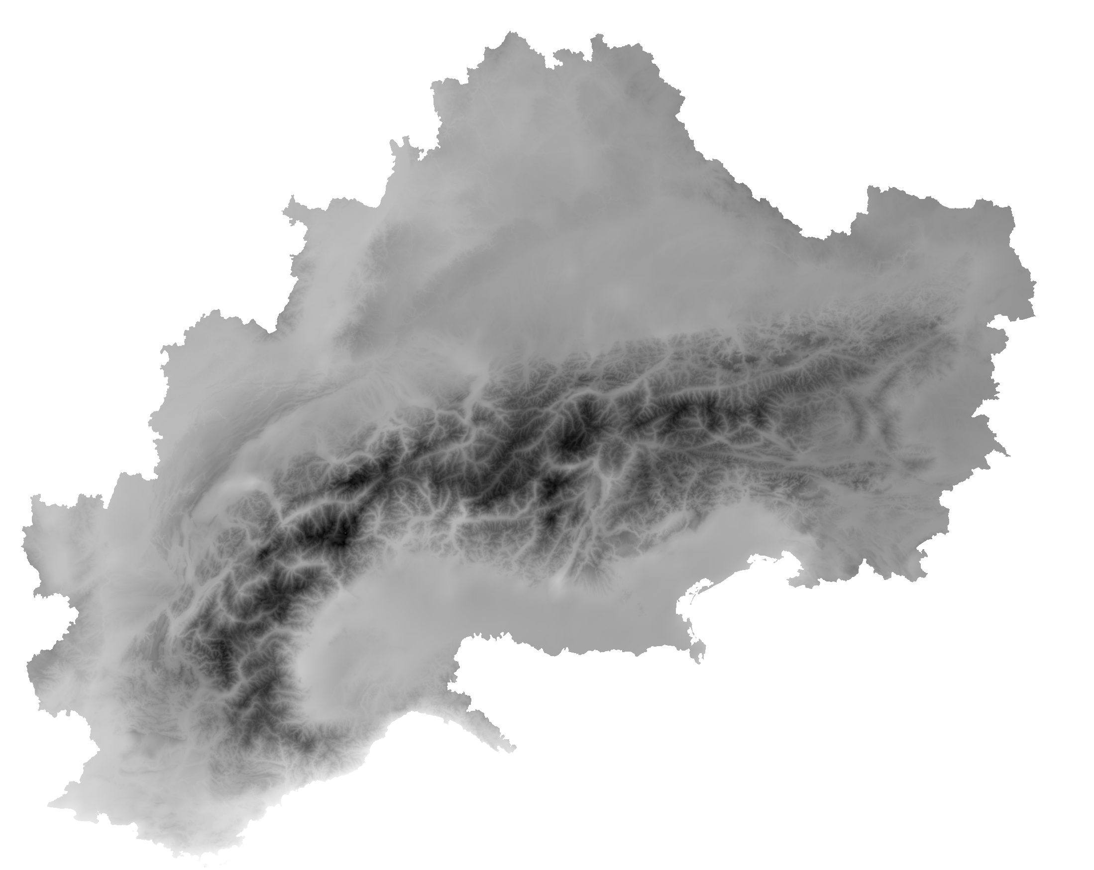
High resolution climatological large ensemble for the Alpine Region
The A-DROP LE is a single model initial condition large ensemble of the Alpine Region. It is based on the Canadian Earth System Model 2 Large Ensemble (CanESM2-LE), that is dynamically downscaled with the Canadian Regional Climate Model (CRCM5) to 12 km spatial resolution (CRCM5-LE) over the European domain (Leduc et al., 2019). It consists of 5 climate variables (air temperature, dew point temperature, precipitation, incoming shortwave radiation and wind speed), that are bias-corrected via MBCn (Cannon, 2018) and statistically downscaled to a spatial resolution of 500 m using the method of Marke, 2008. The temporal resolution is sub-daily (every three hours).
STAC
View
Jan. 1, 1991, 1 a.m.
Dec. 31, 2098, 10 p.m.
Dec. 31, 2098, 10 p.m.
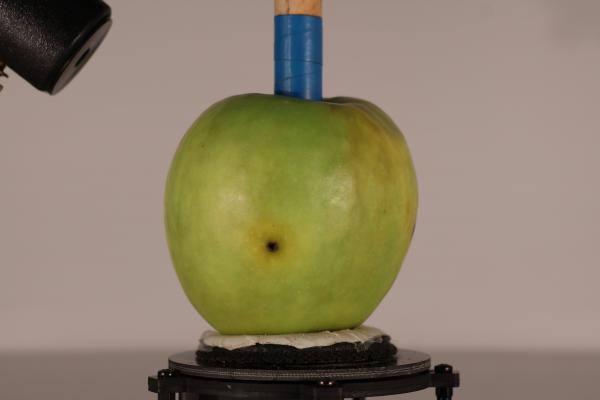
HIPPA - Hyperspectral and RGB imaging of wound-inoculated apples with postharvest pathogens
This collection is part of the HIPPA project, which investigates physiological disorders, mechanical damage and fungal diseases affecting apple fruit at harvest and during postharvest using hyperspectral imaging, RGB imaging and spectroscopy. This collection contains RGB images and hyperspectral images of wound-inoculated apples infected with eight different pathogens and corresponding control samples. Healthy-looking apples were manually surface-sterilized and inoculated with spore suspensions. To cover all cultivars and pathogens, apples were prepared and acquired in groups referred to as 'batches' at different timestamps. Each batch contains apples from one specific cultivar and includes a subset of pathogen treatments together with control samples; each batch generally contains approximately 24 apples per included treatment and approximately 24 control apples. Each STAC Item represents one apple sample at one specific day post-inoculation. Item identifiers follow the pattern apple_{sample_id}_dpi{dpi:02d}, for example apple_57000_dpi03. The acquisition setup is an enclosed space of approximately 1 x 1 m, equipped with a lighting system, a rotating platform and multiple optical instruments measuring the apple surface. Acquisitions are performed in the Eurac Research - Center for Sensing Solutions laboratories. The Collection spatial extent represents the general area of origin of the apple samples, while Item geometries represent the laboratory acquisition location.
STAC
View
Oct. 21, 2024, 2 a.m.
June 27, 2026, 1:59 a.m.
June 27, 2026, 1:59 a.m.
Hunsruck_Hochwald_national_park
This collection is based on Sentinel-2 level 2A dataset acquired from both Sentinel-2 A and B satellites.
It covers a temporal range of 01-02-2021 to 30-09-2023, for every site all Sentinel scenes covering the area are included.
The collection includes all bands at a resolution of 10 meters. The bands are listed below.
B02
B03
B04
B05
B06
B07
B08
B8A
B09
B11
B12
SCL
The Level-2A data includes a Scene Classification, the algorithm allows the detection of clouds, snow and cloud shadows and generation of a classification map.
Cloud screening is applied to the data in order to retrieve accurate atmospheric and surface parameters during the atmospheric correction step.
The L2A SCL map can also be a valuable input for further processing steps or data analysis.
The collection covers all sites of the Hyperecos project. The following sites are included with the spatial extent mentioned.
Cireco {'west': 12.870775000000037, 'east': 13.103782000000024, 'south': 41.22186599400004, 'north': 41.41504699400008}
Orbetello {'west': 11.181888751927033,'east': 11.455397318265538, 'south': 42.372996996314896, 'north': 42.50311599528868}
Sciliar - Catinaccio {'west': 11.506713000000047, 'east': 11.667129000000045, 'south': 46.440615996000076, 'north': 46.54040999600005}
Castel Porziano {'west': 12.345466114000033, 'east': 12.451677663000055, 'south': 41.65575504100008, 'north': 41.78393419900004}
Monte Bondone {'west': 11.027602448000039, 'east': 11.044658587000072, 'south': 45.98801759300005, 'north': 46.01382867600006}
Bosco Fontana {'west': 10.73031770800003, 'east': 10.757708439000055, 'south': 45.192834764000054, 'north': 45.20899297600005}
Hunsrück-Hochwald {"west": 6.98720747225448, "east": 7.28904390300005, "north": 49.7943764377934, "south": 49.60530142600001}
STAC
View
May 2, 2021, 2 a.m.
Sept. 29, 2023, 2 a.m.
Sept. 29, 2023, 2 a.m.
IEQ Monitoring Dataset of a Coastal Hotel in Veneto, Italy (Summer–Autumn 2013)
This dataset contains indoor environmental quality (IEQ) monitoring data collected in a hotel located on the Veneto Adriatic coast (Italy) during summer–autumn 2013. Data were collected at 10-minute intervals across 10 indoor zones (8 guest rooms on 4 floors, bar, and restaurant) and one outdoor weather station. Variables include air temperature (°C), relative humidity (%), and illuminance (lux). The dataset is intended as an open benchmark resource for testing IEQ analytics tools, including thermal comfort assessment and anomaly detection algorithms, particularly within the MODERATE platform (Horizon Europe GA 101069834). LICENSE: CC-BY 4.0 DOI: 10.5281/zenodo.20122432 Related resources: Platform: https://www.moderate.cloud (interactive access, API) Documentation: https://moderate-project.github.io/moderate-docs Source code / tools: https://github.com/MODERATE-Project/ Project website: https://moderate-project.eu Grant Agreement: Horizon Europe GA 101069834 This dataset is released under Creative Commons Attribution 4.0 International (CC BY 4.0). You may use, share, and adapt the data for any purpose, provided you give appropriate credit. If you use this dataset, please cite: C. Pozza (2026). IEQ Monitoring Dataset of a Coastal Hotel in Veneto, Italy (Summer–Autumn 2013). Zenodo. https://doi.org/10.5281/zenodo.20122432Project: MODERATE (Horizon Europe GA 101069834). https://www.moderate.cloud
Other
ViewIEQ monitoring – Residential Apartment, Bolzano, Italy (2026)
IEQ monitoring – Residential Apartment, Bolzano, Italy (2026) Source: SwitchBot app weekly backup ZIP exports. Devices: SwitchBot Meter for temperature & humidity; SwitchBot Smart Radiator Thermostat for the living-room TRV. Sampling interval: ~5 minutes (median). Sensors log on state-change + periodic heartbeat; bursts of readings separated by 1–3 seconds within a polling cycle are rounded/deduped to nearest minute by the pipeline. Period: 2026-02-08 → 2026-05-02 (all seven sensors). LICENSE: CC-BY 4.0 DOI: 10.5281/zenodo.20099209 Related resources: Platform: https://www.moderate.cloud (interactive access, API) Documentation: https://moderate-project.github.io/moderate-docs Source code / tools: https://github.com/MODERATE-Project/ Project website: https://moderate-project.eu Grant Agreement: Horizon Europe GA 101069834 This dataset is released under Creative Commons Attribution 4.0 International (CC BY 4.0). You may use, share, and adapt the data for any purpose, provided you give appropriate credit. If you use this dataset, please cite: C. Pozza (2026). IEQ monitoring – Residential Apartment, Bolzano, Italy (2026). Zenodo. https://doi.org/10.5281/zenodo.20099209Project: MODERATE (Horizon Europe GA 101069834). https://www.moderate.cloud
Other
ViewIndoor Environmental Quality – Residential Apartment, Bolzano, Italy (2023–2026)
Time-series dataset of indoor environmental quality (IEQ) measurements collected at 5-minute intervals from March 2023 to May 2026 in a south-facing living room (25 m²) of a residential apartment in Bolzano, Italy. Data were acquired using a Netatmo HomeCoach sensor and cover four years of continuous monitoring across four CSV files (one per year). Variables include: timestamp, air temperature (°C), relative humidity (%), CO₂ concentration (ppm), noise level (dB), and atmospheric pressure (hPa). The apartment is equipped with radiators for heating and an air conditioning system for cooling. The dataset is suitable for occupancy pattern analysis, thermal comfort studies, indoor air quality benchmarking, and training/validation of building energy or comfort models. LICENSE: CC-BY 4.0DOI: 10.5281/zenodo.20098783 Related resources: Platform: https://www.moderate.cloud (interactive access, API) Documentation: https://moderate-project.github.io/moderate-docs Source code / tools: https://github.com/MODERATE-Project/ Project website: https://moderate-project.eu Grant Agreement: Horizon Europe GA 101069834 This dataset is released under Creative Commons Attribution 4.0 International (CC BY 4.0). You may use, share, and adapt the data for any purpose, provided you give appropriate credit. If you use this dataset, please cite: C. Pozza (2026). Indoor Environmental Quality – Residential Apartment, Bolzano, Italy (2023–2026). Zenodo. https://doi.org/10.5281/zenodo.20098783Project: MODERATE (Horizon Europe GA 101069834). https://www.moderate.cloud
Other
ViewInnovathon MODERATE 2025 - datasets
Materiales para el desarrollo del Innovathon MODERATE en Octubre 2025 en la EPI Gijón Materials for the development of the Innovathon MODERATE in October 2025 at the EPI Gijón
Other
View
INSTINCT - Reflectance spectroradiometry of Drosophila suzukii infestation risk in cherries, harvest 2025
This collection is part of the INSTINCT project and contains reflectance spectra of sweet cherries acquired during the 2025 harvest season to investigate infestation risk caused by Drosophila suzukii. Protocol 2 focused on cherries at an early ripening stage, when susceptibility to infestation was changing. Untreated cherries were collected from net-protected Kordia and Regina orchard rows at Laimburg Research Centre and exposed to Drosophila suzukii. After exposure, each cherry was classified as non-infested, infested, or punctured without oviposition. Each STAC Item represents one cherry measured once. Three reflectance spectra were acquired at random surface points using an SVC HR-1024i spectroradiometer with the LC-RP PRO Leaf Clip and Reflectance Probe and its integrated light source. Measurements were performed in the Eurac Research - Center for Sensing Solutions laboratories. Item geometries represent the laboratory measurement location.
STAC
View
May 27, 2025, 7:39 p.m.
June 10, 2025, 7:56 p.m.
June 10, 2025, 7:56 p.m.
INSTINCT - Reflectance spectroradiometry of Drosophila suzukii infestation status in cherries, harvest 2024
This collection is part of the INSTINCT project and contains reflectance spectra of sweet cherries acquired during the 2024 harvest season to investigate infestation status caused by Drosophila suzukii. Protocol 1 was conducted during the ripening period in which cherries were susceptible to infestation. Untreated and initially non-infested cherries were collected from net-protected orchard rows at Laimburg Research Centre. A subset was exposed to Drosophila suzukii in cages and only correctly infested cherries were retained; an equal group of non-infested control cherries was not exposed in the cages. The same cherries were measured repeatedly at multiple nominal hours after the batch-specific exposure reference time, making the experimental design longitudinal. Each STAC Item represents one cherry at one measurement time. Three reflectance spectra were acquired at random surface points on each cherry using an SVC HR-1024i spectroradiometer with the LC-RP PRO Leaf Clip and Reflectance Probe. Measurements were performed in the Eurac Research - Center for Sensing Solutions laboratories. Item geometries represent the laboratory measurement location. Experimental batches B00 and B01 were preliminary tests and are excluded.
STAC
View
May 30, 2024, 9:26 a.m.
June 27, 2024, 12:07 p.m.
June 27, 2024, 12:07 p.m.
INSTINCT - Reflectance spectroradiometry of Drosophila suzukii infestation status in cherries, harvest 2025
This collection is part of the INSTINCT project and contains reflectance spectra of sweet cherries acquired during the 2025 harvest season to investigate infestation status caused by Drosophila suzukii. Protocol 1 was conducted during the ripening period in which cherries were susceptible to infestation. Untreated and initially non-infested cherries were collected from net-protected orchard rows at Laimburg Research Centre. A subset was exposed to Drosophila suzukii in cages and only correctly infested cherries were retained; an equal group of non-infested control cherries was not exposed in the cages. Different cherries were measured at the different nominal hours after exposure, making the experimental design repeated-timepoint rather than longitudinal. Each STAC Item represents one cherry at one measurement time. Three reflectance spectra were acquired at random surface points on each cherry using an SVC HR-1024i spectroradiometer with the LC-RP PRO Leaf Clip and Reflectance Probe. Measurements were performed in the Eurac Research - Center for Sensing Solutions laboratories. Item geometries represent the laboratory measurement location.
STAC
View
June 5, 2025, 3:08 p.m.
June 25, 2025, 6:42 p.m.
June 25, 2025, 6:42 p.m.
INSTINCT - Transmittance spectroradiometry of Drosophila suzukii infestation risk in cherries, harvest 2025
This collection is part of the INSTINCT project and contains transmittance spectra of sweet cherries acquired during the 2025 harvest season under Protocol 2 to investigate susceptibility to Drosophila suzukii infestation during early fruit maturation. Untreated cherries of the Kordia and Regina cultivars were collected from net-protected orchard rows at Laimburg Research Centre. All cherries were exposed to Drosophila suzukii and subsequently classified as non-infested, infested, or punctured without oviposition. Each STAC Item represents one cherry measured once and contains one transmittance spectrum. Measurements were acquired with an SVC HR-1024i spectroradiometer using a Fresnel Junior 150 W tungsten light source positioned on one side of the fruit and the SVC optical fibre on the opposite side. Measurements were performed in the Eurac Research - Center for Sensing Solutions laboratories. Item geometries represent the laboratory measurement location. Asset SPT-T_B20_H034_C047_0.sig is excluded because no infestation label is available.
STAC
View
May 27, 2025, 8:15 p.m.
June 10, 2025, 8:13 p.m.
June 10, 2025, 8:13 p.m.
INSTINCT - Transmittance spectroradiometry of Drosophila suzukii infestation status in cherries, harvest 2024
This collection is part of the INSTINCT project and contains transmittance spectra of sweet cherries acquired during the 2024 harvest season to investigate infestation status caused by Drosophila suzukii. Protocol 1 was conducted during the ripening period in which cherries were susceptible to infestation. Untreated and initially non-infested cherries were collected from net-protected orchard rows at Laimburg Research Centre. A subset was exposed to Drosophila suzukii in cages and only correctly infested cherries were retained; an equal group of non-infested control cherries was not exposed in the cages. Each STAC Item represents one cherry at one measurement time and contains one transmittance spectrum. Measurements were acquired using an SVC HR-1024i spectroradiometer, with a Fresnel Junior 150 W tungsten light source positioned on one side of the fruit and the SVC optical fibre on the opposite side. Measurements were performed in the Eurac Research - Center for Sensing Solutions laboratories. Item geometries represent the laboratory measurement location. Only batches B10 to B17 are represented in this collection.
STAC
View
June 14, 2024, 3:07 p.m.
June 27, 2024, 12:43 p.m.
June 27, 2024, 12:43 p.m.
INSTINCT - Transmittance spectroradiometry of Drosophila suzukii infestation status in cherries, harvest 2025
This collection is part of the INSTINCT project and contains transmittance spectra of sweet cherries acquired during the 2025 harvest season to investigate infestation status caused by Drosophila suzukii. Protocol 1 was conducted during the ripening period in which cherries were susceptible to infestation. Untreated and initially non-infested cherries were collected from net-protected orchard rows at Laimburg Research Centre. A subset was exposed to Drosophila suzukii in cages and correctly infested cherries were compared with non-infested controls. Different cherries were measured at the represented nominal hours, making the experimental design repeated-timepoint. Each STAC Item represents one cherry at one measurement time and contains one transmittance spectrum. Measurements were acquired using an SVC HR-1024i spectroradiometer, with a Fresnel Junior 150 W tungsten light source positioned on one side of the fruit and the SVC optical fibre on the opposite side. Measurements were performed in the Eurac Research - Center for Sensing Solutions laboratories. Item geometries represent the laboratory measurement location.
STAC
View
June 5, 2025, 3:46 p.m.
June 24, 2025, 5:12 p.m.
June 24, 2025, 5:12 p.m.
LagunaOrbetello
This collection is based on Sentinel-2 level 2A dataset acquired from both Sentinel-2 A and B satellites.
It covers a temporal range of 01-02-2021 to 30-09-2023, for every site all Sentinel scenes covering the area are included.
The collection includes all bands at a resolution of 10 meters. The bands are listed below.
B02
B03
B04
B05
B06
B07
B08
B8A
B09
B11
B12
SCL
The Level-2A data includes a Scene Classification, the algorithm allows the detection of clouds, snow and cloud shadows and generation of a classification map.
Cloud screening is applied to the data in order to retrieve accurate atmospheric and surface parameters during the atmospheric correction step.
The L2A SCL map can also be a valuable input for further processing steps or data analysis.
The collection covers all sites of the Hyperecos project. The following sites are included with the spatial extent mentioned.
Cireco {'west': 12.870775000000037, 'east': 13.103782000000024, 'south': 41.22186599400004, 'north': 41.41504699400008}
Orbetello {'west': 11.181888751927033,'east': 11.455397318265538, 'south': 42.372996996314896, 'north': 42.50311599528868}
Sciliar - Catinaccio {'west': 11.506713000000047, 'east': 11.667129000000045, 'south': 46.440615996000076, 'north': 46.54040999600005}
Castel Porziano {'west': 12.345466114000033, 'east': 12.451677663000055, 'south': 41.65575504100008, 'north': 41.78393419900004}
Monte Bondone {'west': 11.027602448000039, 'east': 11.044658587000072, 'south': 45.98801759300005, 'north': 46.01382867600006}
Bosco Fontana {'west': 10.73031770800003, 'east': 10.757708439000055, 'south': 45.192834764000054, 'north': 45.20899297600005}
Hunsrück-Hochwald {"west": 6.98720747225448, "east": 7.28904390300005, "north": 49.7943764377934, "south": 49.60530142600001}
STAC
View
May 3, 2021, 2 a.m.
Sept. 27, 2023, 2 a.m.
Sept. 27, 2023, 2 a.m.
Land Surface Temperature - 231m 8 day mean
The Land Surface Temperature (LST) is based on MODIS satellite data. The LST is based on 8 day MOD11A2 (v006) LST products. The spatial resolution is 231 m after regridding from the original 1000 m resolution. The LST is masked to the highest quality standards using the provided quality layers. Missing pixel values in the time series are linearly interpolated. Non-vegetatated areas are masked using the MODIS land cover product layer MCD12Q1 FAO-Land Cover Classification System 1 (LCCS1). The final product is regridded to the LAEA Projection (EPSG:3035). The Land Surface Temperature is expressed in degree Celsius.
STAC
View
Jan. 1, 2001, 1 a.m.
Jan. 3, 2021, 1 a.m.
Jan. 3, 2021, 1 a.m.
LEC Location Assessment Dataset – Crevillent (Valencia Region)
This dataset supports the Local Energy Communities (LEC) Location Assessment Tool developed within the MODERATE project (Horizon Europe GA 101069834). It combines cadastral geometry, solar PV potential estimates, sociodemographic indicators, and building stock characteristics at the parcel level for the municipality of Crevillent (Valencia Region, Spain). The dataset was used to train and validate the LEC assessment analytics, enabling identification of optimal areas for the formation of local energy communities based on building morphology, roof-mounted PV capacity, energy demand proxies, and population data. Data sources include the Spanish Cadastre (Sede Electrónica del Catastro) and INE census sections. Tags/Keywords: local energy communities, LEC, solar PV, cadastral data, building stock, Valencia, Spain, energy communities, MODERATE, Horizon Europe, geo-clustering, renewable energy License: CC BY 4.0DOI: 10.5281/zenodo.20121502 Spatial coverage: Municipality of Crevillent, Province of Alicante, Valencia Region, SpainCoordinate reference system: EPSG:25830 (ETRS89 / UTM zone 30N) — geometry column; WGS84 lat/lon also present Related resources: Platform: https://www.moderate.cloud (interactive access, API) Documentation: https://moderate-project.github.io/moderate-docs Source code / tools: https://github.com/MODERATE-Project/ Project website: https://moderate-project.eu Grant Agreement: Horizon Europe GA 101069834 This dataset is released under Creative Commons Attribution 4.0 International (CC BY 4.0). You may use, share, and adapt the data for any purpose, provided you give appropriate credit. If you use this dataset, please cite: E. Guillo Sansano (Grupo Enercoop) - 2026. LEC Location Assessment Dataset – Crevillent (Valencia Region). Zenodo. https://doi.org/10.5281/zenodo.20121502Project: MODERATE (Horizon Europe GA 101069834). https://www.moderate.cloud
Other
View
LiDAR-derived Forest Mapping in Mazia valley
This dataset contains forest structural and species information derived from RGB-colored LiDAR point clouds collected by Eurac Research. Using a standardized R workflow (lidR, ForestTools), the LiDAR data were processed through ground classification, height normalization, canopy height model (CHM) generation, individual tree detection, crown segmentation, point-cloud tree assignment, and RGB-based unsupervised species clustering. The result is a set of spatial layers representing tree locations, tree crowns, canopy structure, and species group labels. These data products support forest monitoring, digital twin development, ecological analysis, and modelling of forest dynamics.
STAC
View
Oct. 22, 2025, 2 a.m.
June 8, 2026, 2 a.m.
June 8, 2026, 2 a.m.
LSTM Representative Dataset for tile 31TFJ - Collected around the fire event in Martigues on August 4, 2020
Representative bands for the Land Surface Temperature Monitoring consolidated within the SENWISE initiative, gathered from sources as Sentinel-2, Sentinel-3 enhanced at high resolution, and simulation alogrithms
STAC
View
July 1, 2020, 11:50 a.m.
Aug. 15, 2020, 12:40 p.m.
Aug. 15, 2020, 12:40 p.m.
MERIT Hydro datasets
MERIT Hydro is a global hydrography datasets, developed based on the MERIT DEM and multiple inland water maps. It contains flow direction, flow accumulation, hydrologically adjusted elevations, and river channel width.
STAC
View
March 1, 2024, 1 a.m.
March 1, 2024, 1 a.m.
March 1, 2024, 1 a.m.
MERIT Hydro datasets for the European Alps
MERIT Hydro is a global hydrography datasets, developed based on the MERIT DEM and multiple inland water maps. It contains flow direction, flow accumulation, hydrologically adjusted elevations, and river channel width.
STAC
View
March 1, 2024, 1 a.m.
March 1, 2024, 1 a.m.
March 1, 2024, 1 a.m.

METER ATMOS 41 all-in-one weather station (A2 Roof Building NOI Techpark, Bolzano - Italy)
This dataset contains meteorological observations recorded by a METER ATMOS 41 all-in-one weather station installed on the roof of Building A2 at NOI Techpark. The main monitoring period began around 2022, and the station remains installed at the site. The recorded variables include solar radiation, precipitation and maximum precipitation rate, lightning activity and distance, wind direction, wind speed and gust speed, air temperature, vapour pressure, vapour pressure deficit, and atmospheric pressure. Additional measurements include the station’s tilt along the X and Y axes, RH sensor temperature, and diagnostic information related to the battery, barometer, and data logger. Observations are generally recorded at 20-minute intervals.
PostgreSQL
View
Oct. 22, 2022, 2 a.m.
Oct. 6, 2026, 2:52 p.m.
Oct. 6, 2026, 2:52 p.m.
MOD10A1 daily snow cover fraction for the Senales valley
This data set provides a daily snow cover fraction derived from the "MODIS/Terra Snow Cover 5-Min L2 Swath 500m" data set (DOI:10.5067/MODIS/MOD10_L2.061). The dataset is reprojected and regridded to a specific area of interest (Senales catchment). The original MODIS snow-cover products provide Normalized Difference Snow Index (NDSI) values from 0 – 100. NDSI is then converted to snow cover fraction (SCF) from 0 – 100 (Salomonson and Appel, 2004; Riggs et al., 2019). Clouds are marked as 205.
STAC
View
Jan. 1, 2016, 1 a.m.
Feb. 1, 2023, 1 a.m.
Feb. 1, 2023, 1 a.m.
MOD16 Evapotranspiration - 500 m
Operational MODIS ET product over the Alps
STAC
View
Jan. 1, 2001, 1 a.m.
Dec. 27, 2019, 1 a.m.
Dec. 27, 2019, 1 a.m.
MODERATE Solar Cadastre Dataset
This dataset contains building and rooftop characteristics for the city of Crevillent , Spain, together with estimated photovoltaic (PV) potential indicators, including suitable roof area, installable PV capacity, expected yearly electricity production, specific PV yield, and potential CO₂ emission savings. The PV potential assessment combines building footprints, annual irradiance data, terrain geometry, and shading analysis using a digital elevation model (DEM), while PV performance is derived from PVGIS and processed with PVLIB. Only technically and economically feasible rooftop areas are included. The dataset includes the following entries: Column Explanation ID Unique identifier of the building or roof section b_area Building or roof subsection area used for the calculation (in m²) p_area Total parcel or roof area associated with the building (m²) building_u Building use / building category year_cons Year of construction floors Number of floors of the building dwellings Number of residential units/apartments r_typology Residential typology thermal_ne Thermal need – Annual thermal energy demand of the building parcel, in MWh/year area_conv Roof area convenient/suitable for PV installation (m²) – this area is used for PV calculations PV_nominal Estimated installed PV peak power (kWp) PV_potential Estimated yearly PV electricity production (kWh/year) average_yi Specific PV yield (kWh/kWp/year) potentialC… Potential annual CO₂ emissions avoided (kg CO₂/year) centroid_l Latitude of building centroid centroid_1 Longitude of building centroid centroid_x X coordinate in projected coordinate system centroid_y Y coordinate in projected coordinate system Derivation of the dataset: The dataset combines building footprints with a spatial annual irradiance raster (e.g., a local solar‑cadastre / processed irradiance layer) and a digital elevation model (DEM) to capture site geometry and shading; hourly PV performance and solar geometry come from PVGIS [1] and are processed with PVLIB [2] for accurate sun positions; PVGIS hourly profiles are horizon‑corrected (using the DEM) and then scaled to match the raster’s annual totals. Finally, a set of internal technical and economic assumptions (module efficiency, performance ratio, self‑consumption/export tariffs, investment cost, discount rate, lifetime, etc.) converts energy into annual revenue and Net Present Value (NPV), and only pixels with positive NPV are considered feasible—producing per‑building feasible area, nominal capacity, annual generation (post‑shading, raster‑calibrated), specific yield, and estimated CO₂. [1] Photovoltaic Geographical Information System (PVGIS), European Commission Joint Research Centre. Available online: https://joint-research-centre.ec.europa.eu/photovoltaic-geographical-information-system-pvgis_en [2] Anderson, K., Hansen, C., Holmgren, W., Jensen, A., Mikofski, M., and Driesse, A. “pvlib python: 2023 project update.” Journal of Open Source Software, 8(92), 5994, (2023). DOI: 10.21105/joss.05994.
Other
ViewMODERATE Synthetic energy consumption profiles
Synthetic dataset with 500 users hourly profile of energy metering data. The original training dataset contains both residential and non residential buildings, from 5000 users. Meaning of the columns: A+: Active energy consumed from the grid (Wh) A-: Active energy exported to the grid (Wh) R1: Consumed inductive reactive energy R2: Generated inductive reactive energy R3: Consumed cpacitive reactive energy R4: Generated capacitive reactive energy NOTE: The two variants "cpu" and "xpu" do not differ statistically from each other. They are both result obtained by MOSTLY.AI library running on a local instance, run with pytorch in the CPU (multi-thread) mode, vs a XPU pytorch run. Specific statistical metrics shows that the synthetic dataset is significantly different from original profiles. While daily and weekly patterns are maintained from the synthetization process set up, in this first release the seasonal and monthly patterns are not represented in the synthetic dataset.
Other
ViewMODERATE Training dataset for synthetic load profile generator
Source: Fluvius Open Data portal Original dataset: Fluvius 2,400 digital meter profiles Description: This dataset contains 15-minute smart meter electricity readings from 2,400 anonymised residential customers connected to the Fluvius distribution network in Flanders, Belgium, covering a full calendar year. Each profile is labelled according to the presence of distributed energy technologies: photovoltaic (PV) systems, electric vehicles (EV), heat pumps (HP), or none of these. For this project, the dataset was resampled to hourly resolution and a subset of 1,300 profiles was selected, resulting in a matrix of 1,300 columns × 8,760 hourly values representing electricity consumption per building. Labels for each profile are provided in a separate indicator file. Use: The dataset was used as the basis for synthetic load profile generation within the MODERATE project.
Other
View
MODIS First Snow Day 500m
FSD represents the first date in the hydrological year with snow presence
STAC
View
Oct. 1, 2000, 2 a.m.
Sept. 30, 2023, 2 a.m.
Sept. 30, 2023, 2 a.m.

MODIS Last Snow Day 500m
LSD represents the last date in the hydrological year with snow presence
STAC
View
Oct. 1, 2000, 2 a.m.
Sept. 30, 2023, 2 a.m.
Sept. 30, 2023, 2 a.m.
MODIS Leaf Area Index
The MCD15A3H Version 6.1 Moderate Resolution Imaging Spectroradiometer (MODIS) Level 4 Leaf Area Index (LAI) product is a 4-day composite data set with 500 meter pixel size. The algorithm chooses the best pixel available from all the acquisitions of both MODIS sensors located on NASA’s Terra and Aqua satellites from within the 4-day period. LAI is defined as the one-sided green leaf area per unit ground area in broadleaf canopies and as one-half the total needle surface area per unit ground area in coniferous canopies.
STAC
View
Jan. 1, 2020, 1 a.m.
Dec. 1, 2020, 1 a.m.
Dec. 1, 2020, 1 a.m.

MODIS Snow Cover Area 500m
The yearly snow cover area derived derived from daily MOD10A1 images
STAC
View
Oct. 1, 2000, 2 a.m.
Sept. 30, 2023, 2 a.m.
Sept. 30, 2023, 2 a.m.

MODIS Snow Cover Duration 500m
The yearly snow cover duration derived from daily MOD10A1 images indicationg the number of days with snow presence in one hydrological year
STAC
View
Oct. 1, 2000, 2 a.m.
Sept. 30, 2023, 2 a.m.
Sept. 30, 2023, 2 a.m.
MODIS SNOW map over the ALPS
The collection contains binary snow cover maps covering the entire Alpine Arc. The maps have a daily frequency and a ground resolution of 250 m. They are derived from daily MODIS observations (Aqua and Terra) for the entire Alps arc. The input data are the atmospherically-corrected reflectances of MODIS MOD09GQ, MOD09GA for tile h19v04 and h18v04. The map has two bands - SNOW MAP: Snow cover classification map with four classes [0 = NO DATA - missing or corrupt data of one or more input bands; 1 = SNOW - pixel covered by snow; 2 = NO_SNOW - pixel not covered by snow; 3 = CLOUD - pixel covered by clouds; 4 = OCEAN WATER - pixel over sea and ocean; 5 = INLAND WATER - pixel over lakes and rivers], QUALITY FLAG: Snow cover quality map [NO DATA - missing or corrupt data of one or more input bands; QUALITY_INDEX - higher values indicate higher likeliness of correct classification].
STAC
View
July 3, 2002, 2 p.m.
None
None
MonteBondone
This collection is based on Sentinel-2 level 2A dataset acquired from both Sentinel-2 A and B satellites.
It covers a temporal range of 01-02-2021 to 30-09-2023, for every site all Sentinel scenes covering the area are included.
The collection includes all bands at a resolution of 10 meters. The bands are listed below.
B02
B03
B04
B05
B06
B07
B08
B8A
B09
B11
B12
SCL
The Level-2A data includes a Scene Classification, the algorithm allows the detection of clouds, snow and cloud shadows and generation of a classification map.
Cloud screening is applied to the data in order to retrieve accurate atmospheric and surface parameters during the atmospheric correction step.
The L2A SCL map can also be a valuable input for further processing steps or data analysis.
The collection covers all sites of the Hyperecos project. The following sites are included with the spatial extent mentioned.
Cireco {'west': 12.870775000000037, 'east': 13.103782000000024, 'south': 41.22186599400004, 'north': 41.41504699400008}
Orbetello {'west': 11.181888751927033,'east': 11.455397318265538, 'south': 42.372996996314896, 'north': 42.50311599528868}
Sciliar - Catinaccio {'west': 11.506713000000047, 'east': 11.667129000000045, 'south': 46.440615996000076, 'north': 46.54040999600005}
Castel Porziano {'west': 12.345466114000033, 'east': 12.451677663000055, 'south': 41.65575504100008, 'north': 41.78393419900004}
Monte Bondone {'west': 11.027602448000039, 'east': 11.044658587000072, 'south': 45.98801759300005, 'north': 46.01382867600006}
Bosco Fontana {'west': 10.73031770800003, 'east': 10.757708439000055, 'south': 45.192834764000054, 'north': 45.20899297600005}
Hunsrück-Hochwald {"west": 6.98720747225448, "east": 7.28904390300005, "north": 49.7943764377934, "south": 49.60530142600001}
STAC
View
May 1, 2021, 2 a.m.
Sept. 28, 2023, 2 a.m.
Sept. 28, 2023, 2 a.m.
Multi-Family Residential Building – Hourly Energy and IEQ Monitoring Time Series - Bolzano area, Italy (2006–2009)
This dataset contains three years of hourly monitored data from a multi-family residential building located in the Bolzano area, South Tyrol, Italy (46°N, Alpine climate). It covers the period from 1 July 2006 to 21 July 2009 and provides continuous time series combining energy consumption measurements with indoor environmental quality (IEQ) indicators and meteorological context variables. The dataset is released as original monitored data: no outlier removal, smoothing, or gap-filling has been applied. A number of anomalous values and atypical operational trends have been intentionally preserved. This makes the dataset well-suited for benchmarking and stress-testing anomaly detection algorithms, fault detection and diagnostics (FDD) tools, and data quality assessment pipelines in the building energy domain. Note: Temperature profiles are obtained after averaging on similar profiles from 8 selected apartments. The energy consumption is the aggregated value at building level (same apartments). Variable Description Unit Min Max Mean Electricity Hourly electrical energy consumption kWh 0.00 78.00 1.62 CO₂ concentration Indoor CO₂ concentration (occupancy/ventilation proxy) ppm 452 1908 832.71 Internal temperature Indoor air temperature °C 12.60 31.20 24.27 Thermal energy consumption Hourly thermal energy (heating/DHW) kWh 0.00 27.00 5.98 External global radiation Horizontal global solar irradiance W/m² 0.00 1035.00 151.95 Outside temperature Outdoor ambient air temperature °C −8.10 38.30 13.33 Note: min, max, and mean are computed over all 25,699 records. No missing values are present. Extreme values (e.g., electricity max 78 kWh/h; CO₂ max 1,908 ppm) reflect both real operational peaks and intentionally retained anomalous readings. Users should not treat these values as errors before understanding the anomaly detection context of this release. Related resources: Platform: https://www.moderate.cloud (interactive access, API) Documentation: https://moderate-project.github.io/moderate-docs Source code / tools: https://github.com/MODERATE-Project/ Project website: https://moderate-project.eu Grant Agreement: Horizon Europe GA 101069834 This dataset is released under Creative Commons Attribution 4.0 International (CC BY 4.0). You may use, share, and adapt the data for any purpose, provided you give appropriate credit. If you use this dataset, please cite: M. Castagna, C. Pozza (2026). Multi-Family Residential Building – Hourly Energy and IEQ Monitoring Time Series - Bolzano area, Italy (2006–2009). Zenodo. https://doi.org/10.5281/zenodo.20096697Project: MODERATE (Horizon Europe GA 101069834). https://www.moderate.cloud
Other
View
Normalized Difference Vegetation Index - 231m 8 day Maximum Value Composite
The Normalized Difference Vegetation Index (NDVI) is based on MODIS satellite data. The NDVI is based on 8 day maximum value composite MOD09Q1 (v006) reflectance products. The spatial resolution is 231 m. The NDVI is masked to the highest quality standards using the provided quality layers. Missing pixel values in the time series are linearly interpolated. Non-vegetatated areas are masked using the MODIS land cover product layer MCD12Q1 FAO-Land Cover Classification System 1 (LCCS1). The final product is regridded to the LAEA Projection (EPSG:3035). The NDVI is calculated using the formula NDVI = (NIR - Red) / (NIR + Red). The NDVI expresses the vitality of vegetation. The data is provided as 8 day measures. The time series is starting from 2001. The NDVI values range from -1 - 1, whereas high values correspond to healthy vegetation.
STAC
View
Jan. 1, 2001, 1 a.m.
Jan. 3, 2021, 1 a.m.
Jan. 3, 2021, 1 a.m.
Ospitaletto District Heating Expansion – Building Heat Demand and Network Dataset
This dataset provides georeferenced building-level annual heating demand estimates and district heating network geometry for the municipality of Ospitaletto (Brescia, Lombardy, Italy), developed to assess expansion opportunities for an existing 5th Generation District Heating (5GDHC) network. The building heat demand layer (Ospitaletto_heat.gpkg) covers 1,957 buildings with 17 attributes including footprint area, building height and volume, S/V ratio, functional use (residential/non-residential), INSPIRE-based typological class (SFH, s-MFH, l-MFH), estimated annual heating demand (MWh/year), distance to the DH network, and priority selection flags under two criteria. The DH network layer (DH_ospitaletto_network.gpkg) contains 21 pipe segments of the existing network. Both layers use the EPSG:3035 coordinate reference system. Heating demand was estimated through a data-fusion methodology combining building geometry (OpenStreetMap, cadastral data), climate inputs (Heating Degree Days, Southern Continental zone), energy consumption density benchmarks (INSPIRE for residential, Hotmaps for non-residential), and available metered consumption data for calibration. Network expansion priorities were assessed using two criteria: Criterion A selects buildings by maximizing the ratio of annual demand to distance from the network (kWh/y/m); Criterion B applies a 250 m buffer around the existing network and filters by minimum demand threshold (100 kWh/y). Produced within the MODERATE project (Horizon Europe Grant Agreement No. 101069834).
Other
View
Precipitation Anomalies - ERA5_QM REL_RR-1
Relative precipitation anomalies are based on downscaled ERA5 reanalysis data (downscaling is performed using quantile mapping method) and calculated for different time scales (1, 2, 3, 6, 12 months). The values represent the % of normal precipitation, where normal is defined as the long-term average (1981-2020).
STAC
View
Dec. 31, 1978, 1 p.m.
None
None
Precipitation Anomalies - ERA5_QM REL_RR-12
Relative precipitation anomalies are based on downscaled ERA5 reanalysis data (downscaling is performed using quantile mapping method) and calculated for different time scales (1, 2, 3, 6, 12 months). The values represent the % of normal precipitation, where normal is defined as the long-term average (1981-2020).
STAC
View
Dec. 31, 1978, 1 p.m.
None
None
Precipitation Anomalies - ERA5_QM REL_RR-2
Relative precipitation anomalies are based on downscaled ERA5 reanalysis data (downscaling is performed using quantile mapping method) and calculated for different time scales (1, 2, 3, 6, 12 months). The values represent the % of normal precipitation, where normal is defined as the long-term average (1981-2020).
STAC
View
Dec. 31, 1978, 1 p.m.
None
None
Precipitation Anomalies - ERA5_QM REL_RR-3
Relative precipitation anomalies are based on downscaled ERA5 reanalysis data (downscaling is performed using quantile mapping method) and calculated for different time scales (1, 2, 3, 6, 12 months). The values represent the % of normal precipitation, where normal is defined as the long-term average (1981-2020).
STAC
View
Dec. 31, 1978, 1 p.m.
None
None
Precipitation Anomalies - ERA5_QM REL_RR-6
Relative precipitation anomalies are based on downscaled ERA5 reanalysis data (downscaling is performed using quantile mapping method) and calculated for different time scales (1, 2, 3, 6, 12 months). The values represent the % of normal precipitation, where normal is defined as the long-term average (1981-2020).
STAC
View
Dec. 31, 1978, 1 p.m.
None
None
PV classification results for the MODERATE project
The csv files contain the results of an image classifier, trained to classify images of rooftops of having or not having PV. It was used on the regions Valencia and Bolzano. The IDs are the building identifiers from Open Street Maps and the prediction classifies each building as having a PV (1) or not having a PV (0). In the respective .json file for each region the latitude and longitude are saved for each Open Street Maps ID using EPSG 3035.
Other
View
RoseL-like DEM differencing, Aix-en-Provence_Pennes-Mirabeau, FR 3, 2025
The RoseL-like DEM difference results of differentiating the X-band Copernicus DEM and an L-band Interferometric DEM built from InSAR processing of the SAOCOM-1B time series acquired during the period from November 2024 to September 2025. Data cover the Aix-en-Provence region, in South of France, including the Pennes-Mirabeau area, where wildfires happened in Summer 2025. Coordinates are [5.094, 43.656], [5.995, 42.999]. With the assumption that the InSAR DEM corresponds to the DTM (i.e. assuming the L-band SAR signal fully reaches the soil, i.e. it is not affected by moisture effects), the result of differencing both DEM's could be considered as a rough proxy of forest height.
STAC
View
Nov. 13, 2024, 1 a.m.
Sept. 29, 2025, 2 a.m.
Sept. 29, 2025, 2 a.m.
RoseL-like DEM differencing, GrandLeez, BE, 2022
The RoseL-like DEM difference results of differentiating the X-band Copernicus DEM and an L-band Interferometric DEM built from InSAR processing of the SAOCOM-1A time series acquired during the period from July to December 2022. Coordinates are [4.726,50.622], [4.85,50.567]. Data cover part of the Walloon Region, in Belgium, including the Forest of Grand-Leez. With the assumption that the InSAR DEM corresponds to the DTM (i.e. assuming the L-band SAR signal fully reaches the soil, i.e. it is not affected by moisture effects), the result of differencing both DEM's could be considered as a rough proxy of forest height.
STAC
View
July 30, 2022, 2 a.m.
Dec. 21, 2022, 1 a.m.
Dec. 21, 2022, 1 a.m.
RoseL-like DEM differencing, Martigues, FR 1, 2025
The RoseL-like DEM difference results of differentiating the X-band Copernicus DEM and an L-band Interferometric DEM built from InSAR processing of the SAOCOM-1A time series acquired during the period from November 2024 to September 2025.Data cover the Martigues area, South of France, where a wildfire happened in Summer 2025. Coordinates are [4.426, 43.55], [5.266, 43.312]. With the assumption that the InSAR DEM corresponds to the DTM (i.e. assuming the L-band SAR signal fully reaches the soil, i.e. it is not affected by moisture effects), the result of differencing both DEM's could be considered as a rough proxy of forest height.
STAC
View
Nov. 14, 2024, 1 a.m.
Sept. 30, 2025, 2 a.m.
Sept. 30, 2025, 2 a.m.
RT1 Surface Soil Moisture - 1 Km
A experimental dataset of soil-moisture retrievals at 1km effective spatial resolution for all 28 basins of the Mediterranean study-area. The data was processed via the RT1 radiative transfer model using Sentinel-1 (VV) backscatter data together with auxiliary CGLS Leaf Area Index timeseries.
STAC
View
Jan. 1, 2017, 1 a.m.
June 30, 2022, 2 a.m.
June 30, 2022, 2 a.m.
SCF_binary
Results for batch job j-2406072110944ac9ae59a2fb48d47a10 (SCF_Binary Map CDSE)
STAC
View
Oct. 1, 2015, 2 a.m.
Sept. 30, 2022, 2 a.m.
Sept. 30, 2022, 2 a.m.
Sciliar_Catinaccio
This collection is based on Sentinel-2 level 2A dataset acquired from both Sentinel-2 A and B satellites.
It covers a temporal range of 01-02-2021 to 30-09-2023, for every site all Sentinel scenes covering the area are included.
The collection includes all bands at a resolution of 10 meters. The bands are listed below.
B02
B03
B04
B05
B06
B07
B08
B8A
B09
B11
B12
SCL
The Level-2A data includes a Scene Classification, the algorithm allows the detection of clouds, snow and cloud shadows and generation of a classification map.
Cloud screening is applied to the data in order to retrieve accurate atmospheric and surface parameters during the atmospheric correction step.
The L2A SCL map can also be a valuable input for further processing steps or data analysis.
The collection covers all sites of the Hyperecos project. The following sites are included with the spatial extent mentioned.
Cireco {'west': 12.870775000000037, 'east': 13.103782000000024, 'south': 41.22186599400004, 'north': 41.41504699400008}
Orbetello {'west': 11.181888751927033,'east': 11.455397318265538, 'south': 42.372996996314896, 'north': 42.50311599528868}
Sciliar - Catinaccio {'west': 11.506713000000047, 'east': 11.667129000000045, 'south': 46.440615996000076, 'north': 46.54040999600005}
Castel Porziano {'west': 12.345466114000033, 'east': 12.451677663000055, 'south': 41.65575504100008, 'north': 41.78393419900004}
Monte Bondone {'west': 11.027602448000039, 'east': 11.044658587000072, 'south': 45.98801759300005, 'north': 46.01382867600006}
Bosco Fontana {'west': 10.73031770800003, 'east': 10.757708439000055, 'south': 45.192834764000054, 'north': 45.20899297600005}
Hunsrück-Hochwald {"west": 6.98720747225448, "east": 7.28904390300005, "north": 49.7943764377934, "south": 49.60530142600001}
STAC
View
May 1, 2021, 2 a.m.
Sept. 28, 2023, 2 a.m.
Sept. 28, 2023, 2 a.m.
Sentinel-2 tiny sample collection for testing purposes.
Tiny sample Sentinel-2 data collection (different dimension names for temporal (time) and bands (band) compared to the SENTINEL2_L2A_SAMPLE collection), generated using openEO, stored initially as netCDF and splitted later into separate COGs (one for each band and each date) for more interoperability.
STAC
View
June 2, 2022, 2 a.m.
June 30, 2022, 2 a.m.
June 30, 2022, 2 a.m.
Sentinel-2 tiny sample collection for testing purposes.
Tiny sample Sentinel-2 data collection, generated using openEO, stored initially as netCDF and splitted later into separate COGs (one for each band and each date) for more interoperability.
STAC
View
June 2, 2022, 2 a.m.
June 30, 2022, 2 a.m.
June 30, 2022, 2 a.m.
SENWISE Input LSTM Representative Dataset
Representative bands for the Land Surface Temperature Monitoring consolidated within the SENWISE initiative, gathered from sources as Sentinel-2, Sentinel-3 enhanced at high resolution, and simulation alogrithms
STAC
View
July 6, 2020, 12:22 p.m.
July 6, 2020, 12:40 p.m.
July 6, 2020, 12:40 p.m.
Snow depth - Venosta Valley
Daily snow depth [mm] maps for the Venosta Valley (South Tyrol,Italy) produced with the GEOtop hydrological model.
STAC
View
Sept. 2, 2019, 2 a.m.
Aug. 2, 2020, 2 a.m.
Aug. 2, 2020, 2 a.m.
SoilGrids data for the European Alps
SoilGrids is a system for global digital soil mapping that uses state-of-the-art machine learning methods to map the spatial distribution of soil properties across the globe. SoilGrids prediction models are fitted using over 230 000 soil profile observations from the WoSIS database and a series of environmental covariates. Covariates were selected from a pool of over 400 environmental layers from Earth observation derived products and other environmental information including climate, land cover and terrain morphology. The outputs of SoilGrids are global soil property maps at six standard depth intervals (according to the GlobalSoilMap IUSS working group and its specifications) at a spatial resolution of 250 meters.
STAC
View
March 1, 2020, 1 a.m.
March 1, 2020, 1 a.m.
March 1, 2020, 1 a.m.

Soil Moisture Anomalies - ERA5_QM
The Soil Moisture Anomaly is a drought indicator used to detect and monitor agricultural drought conditions, defined by a prolonged period of deficit in the availability of soil moisture to plants. The soil moisture anomalies provided as part of the Alpine Drought Observatory was derived from ERA5 Volumetric Soil Water Layers at different depths with Layer 1 (0-7cm), Layer 2 (7-28cm), Layer 3 (28–100cm), and Layer 4 (100-289cm). The input ERA5 soil moisture dataset was downscaled using a quantile mapping approach. Daily anomalies were calculated using a climatological mean and standard deviation of soil moisture from a smoothed time-series (running mean on a 10-day window) for a reference period of 1981–2020. The Soil Moisture Anomalies values range from -5 to +5, with negative values indicating drier than conditions while positive values indicate wetter than normal conditions, and -1 to +1 values indicates near-normal conditions. Datasets contains modified Copernicus Climate Change Service Information [1980–current year]; contains modified Copernicus Atmosphere Monitoring Service Information [1980-current year]. Neither the European Commission nor ECMWF is responsible for any use that may be made of the Copernicus information or data it contains.
STAC
View
Dec. 31, 1979, 1 p.m.
None
None
SSEBop Evapotranspiration - 1 km
Operational FEWS NET ET product over the Alps
STAC
View
Jan. 11, 2003, 1 a.m.
Feb. 1, 2020, 1 a.m.
Feb. 1, 2020, 1 a.m.
Standardised Precipitation-Evapotranspiration Index - ERA5_QM SPEI-1
The Standardized Precipitation-Evapotranspiration Index (SPEI) represents a standardized measure of what a certain value of surface water balance (precipitation minus potential evapotranspiration) over the selected time period means in relation to expected value of surface water balance for this period. SPEI is calculated on different time scales (1, 2, 3, 6, 12 months). The value of the SPEI index around 0 represents the normal expected conditions for the surface water balance in the selected period based on the long-term average (1981-2020). The value of 1 represents approximately one standard deviation of the surplus in the surface water balance, while the value of -1 is about one standard deviation of the deficit. Drought is usually defined as period when SPEI values fall below -1. Input precipitation data is downscaled from ERA5 reanalysis using quantile mapping. Contains modified Copernicus Climate Change Service information [1978-current year]; Contains modified Copernicus Atmosphere Monitoring Service information [1978-current year].
STAC
View
Dec. 31, 1978, 1 p.m.
None
None
Standardised Precipitation-Evapotranspiration Index - ERA5_QM SPEI-12
The Standardized Precipitation-Evapotranspiration Index (SPEI) represents a standardized measure of what a certain value of surface water balance (precipitation minus potential evapotranspiration) over the selected time period means in relation to expected value of surface water balance for this period. SPEI is calculated on different time scales (1, 2, 3, 6, 12 months). The value of the SPEI index around 0 represents the normal expected conditions for the surface water balance in the selected period based on the long-term average (1981-2020). The value of 1 represents approximately one standard deviation of the surplus in the surface water balance, while the value of -1 is about one standard deviation of the deficit. Drought is usually defined as period when SPEI values fall below -1. Input precipitation data is downscaled from ERA5 reanalysis using quantile mapping. Contains modified Copernicus Climate Change Service information [1978-current year]; Contains modified Copernicus Atmosphere Monitoring Service information [1978-current year].
STAC
View
Dec. 31, 1978, 1 p.m.
None
None
Standardised Precipitation-Evapotranspiration Index - ERA5_QM SPEI-2
The Standardized Precipitation-Evapotranspiration Index (SPEI) represents a standardized measure of what a certain value of surface water balance (precipitation minus potential evapotranspiration) over the selected time period means in relation to expected value of surface water balance for this period. SPEI is calculated on different time scales (1, 2, 3, 6, 12 months). The value of the SPEI index around 0 represents the normal expected conditions for the surface water balance in the selected period based on the long-term average (1981-2020). The value of 1 represents approximately one standard deviation of the surplus in the surface water balance, while the value of -1 is about one standard deviation of the deficit. Drought is usually defined as period when SPEI values fall below -1. Input precipitation data is downscaled from ERA5 reanalysis using quantile mapping. Contains modified Copernicus Climate Change Service information [1978-current year]; Contains modified Copernicus Atmosphere Monitoring Service information [1978-current year].
STAC
View
Dec. 31, 1978, 1 p.m.
None
None
Standardised Precipitation-Evapotranspiration Index - ERA5_QM SPEI-3
The Standardized Precipitation-Evapotranspiration Index (SPEI) represents a standardized measure of what a certain value of surface water balance (precipitation minus potential evapotranspiration) over the selected time period means in relation to expected value of surface water balance for this period. SPEI is calculated on different time scales (1, 2, 3, 6, 12 months). The value of the SPEI index around 0 represents the normal expected conditions for the surface water balance in the selected period based on the long-term average (1981-2020). The value of 1 represents approximately one standard deviation of the surplus in the surface water balance, while the value of -1 is about one standard deviation of the deficit. Drought is usually defined as period when SPEI values fall below -1. Input precipitation data is downscaled from ERA5 reanalysis using quantile mapping. Contains modified Copernicus Climate Change Service information [1978-current year]; Contains modified Copernicus Atmosphere Monitoring Service information [1978-current year].
STAC
View
Dec. 31, 1978, 1 p.m.
None
None
Standardised Precipitation-Evapotranspiration Index - ERA5_QM SPEI-6
The Standardized Precipitation-Evapotranspiration Index (SPEI) represents a standardized measure of what a certain value of surface water balance (precipitation minus potential evapotranspiration) over the selected time period means in relation to expected value of surface water balance for this period. SPEI is calculated on different time scales (1, 2, 3, 6, 12 months). The value of the SPEI index around 0 represents the normal expected conditions for the surface water balance in the selected period based on the long-term average (1981-2020). The value of 1 represents approximately one standard deviation of the surplus in the surface water balance, while the value of -1 is about one standard deviation of the deficit. Drought is usually defined as period when SPEI values fall below -1. Input precipitation data is downscaled from ERA5 reanalysis using quantile mapping. Contains modified Copernicus Climate Change Service information [1978-current year]; Contains modified Copernicus Atmosphere Monitoring Service information [1978-current year].
STAC
View
Dec. 31, 1978, 1 p.m.
None
None
Standardised Precipitation Index - ERA5_QM SPI-1
The Standardized Precipitation Index (SPI) represents a standardized measure of what a certain amount of precipitation over the selected time period means in relation to expected amount of precipitation for this period. SPI is used on different time scales (1, 2, 3, 6, 12 months). The value of the SPI index around 0 represents the normal expected conditions regarding the amount of precipitation in the selected time scale compared to the long-term average (1981-2020). Value 1 represents approximately one standard deviation of precipitation amount during wet conditions and -1 denotes about one standard deviation of precipitation amount during dry conditions. Drought is usually defined as period when SPI values fall below -1. Input precipitation data is downscaled from ERA5 reanalysis using quantile mapping. Contains modified Copernicus Climate Change Service information [1978-current year]; Contains modified Copernicus Atmosphere Monitoring Service information [1978-current year].
STAC
View
Dec. 31, 1978, 1 p.m.
None
None
Standardised Precipitation Index - ERA5_QM SPI-12
The Standardized Precipitation Index (SPI) represents a standardized measure of what a certain amount of precipitation over the selected time period means in relation to expected amount of precipitation for this period. SPI is used on different time scales (1, 2, 3, 6, 12 months). The value of the SPI index around 0 represents the normal expected conditions regarding the amount of precipitation in the selected time scale compared to the long-term average (1981-2020). Value 1 represents approximately one standard deviation of precipitation amount during wet conditions and -1 denotes about one standard deviation of precipitation amount during dry conditions. Drought is usually defined as period when SPI values fall below -1. Input precipitation data is downscaled from ERA5 reanalysis using quantile mapping. Contains modified Copernicus Climate Change Service information [1978-current year]; Contains modified Copernicus Atmosphere Monitoring Service information [1978-current year].
STAC
View
Dec. 31, 1978, 1 p.m.
None
None
Standardised Precipitation Index - ERA5_QM SPI-2
The Standardized Precipitation Index (SPI) represents a standardized measure of what a certain amount of precipitation over the selected time period means in relation to expected amount of precipitation for this period. SPI is used on different time scales (1, 2, 3, 6, 12 months). The value of the SPI index around 0 represents the normal expected conditions regarding the amount of precipitation in the selected time scale compared to the long-term average (1981-2020). Value 1 represents approximately one standard deviation of precipitation amount during wet conditions and -1 denotes about one standard deviation of precipitation amount during dry conditions. Drought is usually defined as period when SPI values fall below -1. Input precipitation data is downscaled from ERA5 reanalysis using quantile mapping. Contains modified Copernicus Climate Change Service information [1978-current year]; Contains modified Copernicus Atmosphere Monitoring Service information [1978-current year].
STAC
View
Dec. 31, 1978, 1 p.m.
None
None
Standardised Precipitation Index - ERA5_QM SPI-3
The Standardized Precipitation Index (SPI) represents a standardized measure of what a certain amount of precipitation over the selected time period means in relation to expected amount of precipitation for this period. SPI is used on different time scales (1, 2, 3, 6, 12 months). The value of the SPI index around 0 represents the normal expected conditions regarding the amount of precipitation in the selected time scale compared to the long-term average (1981-2020). Value 1 represents approximately one standard deviation of precipitation amount during wet conditions and -1 denotes about one standard deviation of precipitation amount during dry conditions. Drought is usually defined as period when SPI values fall below -1. Input precipitation data is downscaled from ERA5 reanalysis using quantile mapping. Contains modified Copernicus Climate Change Service information [1978-current year]; Contains modified Copernicus Atmosphere Monitoring Service information [1978-current year].
STAC
View
Dec. 31, 1978, 1 p.m.
None
None
Standardised Precipitation Index - ERA5_QM SPI-6
The Standardized Precipitation Index (SPI) represents a standardized measure of what a certain amount of precipitation over the selected time period means in relation to expected amount of precipitation for this period. SPI is used on different time scales (1, 2, 3, 6, 12 months). The value of the SPI index around 0 represents the normal expected conditions regarding the amount of precipitation in the selected time scale compared to the long-term average (1981-2020). Value 1 represents approximately one standard deviation of precipitation amount during wet conditions and -1 denotes about one standard deviation of precipitation amount during dry conditions. Drought is usually defined as period when SPI values fall below -1. Input precipitation data is downscaled from ERA5 reanalysis using quantile mapping. Contains modified Copernicus Climate Change Service information [1978-current year]; Contains modified Copernicus Atmosphere Monitoring Service information [1978-current year].
STAC
View
Dec. 31, 1978, 1 p.m.
None
None
Standardised Snow Pack Index - ERA5_QM SSPI-10
The Standardized Snow Pack Index (SSPI) represents a standardized measure of what a certain value of snow water equivalent (SWE) averaged over the selected time period means in relation to the expected value for this period. SSPI is computed the same way as the SPI (using gamma distribution), except for being based on daily SWE timeseries instead of daily precipitation. It is calculated using the average SWE over a period of 10 and 30 days. The value of the SSPI index around 0 represents the normal expected conditions for the average SWE in the selected period based on the long-term average (1981-2020). The value of 1 represents approximately one standard deviation of the surplus, while the value of -1 is about one standard deviation of the deficit. SWE data used as input for the calculation of SSPI are derived using a modified version of the deterministic snow model SNOWGRID-CL, with downscaled ERA5 data used as model input data. Contains modified Copernicus Climate Change Service information [1978-current year]; Contains modified Copernicus Atmosphere Monitoring Service information [1978-current year].
STAC
View
Dec. 31, 1978, 1 p.m.
None
None
Standardised Snow Pack Index - ERA5_QM SSPI-30
The Standardized Snow Pack Index (SSPI) represents a standardized measure of what a certain value of snow water equivalent (SWE) averaged over the selected time period means in relation to the expected value for this period. SSPI is computed the same way as the SPI (using gamma distribution), except for being based on daily SWE timeseries instead of daily precipitation. It is calculated using the average SWE over a period of 10 and 30 days. The value of the SSPI index around 0 represents the normal expected conditions for the average SWE in the selected period based on the long-term average (1981-2020). The value of 1 represents approximately one standard deviation of the surplus, while the value of -1 is about one standard deviation of the deficit. SWE data used as input for the calculation of SSPI are derived using a modified version of the deterministic snow model SNOWGRID-CL, with downscaled ERA5 data used as model input data. Contains modified Copernicus Climate Change Service information [1978-current year]; Contains modified Copernicus Atmosphere Monitoring Service information [1978-current year].
STAC
View
Dec. 31, 1978, 1 p.m.
None
None
ST_GRIDDED_TIME_SERIES_PRECIPITATION
The product contains the gridded daily series of mean precipitation at 250-m spatial resolution for the region Trentino – South Tyrol. The dataset was obtained by interpolating on a 250-m resolution grid the observed monthly climatologies of more than 200 station sites of the regional meteorological network and some extra-regional sites close to the borders. All observation data used for deriving the gridded fields were prior checked for quality and homogeneity and they are stored in the Climate Database: https://edp-portal.eurac.edu/cdb_doc/. The climatologies refer to the averages over a reference 30-year period. Further details can be found in the published paper (Crespi et al., 2021; https://doi.org/10.5194/essd-13-2801-2021). The dataset is also available in PANGAEA repository.
STAC
View
Jan. 1, 2020, 1 p.m.
Jan. 1, 2023, 1 p.m.
Jan. 1, 2023, 1 p.m.
ST_GRIDDED_TIME_SERIES_TEMPERATURE
The product contains the gridded daily series of mean temperature at 250-m spatial resolution for the region Trentino – South Tyrol. The dataset currently spans the period 1980 – 2020, but it is expected to be regularly updated. It was obtained by applying an anomaly-based interpolation to the observations of more than 200 station sites of the regional meteorological network and some extra-regional sites close to the borders. All station series used for deriving the gridded fields were prior checked for quality and homogeneity and they are stored in the Climate Database: https://edp-portal.eurac.edu/cdb_doc/. Mean temperature was here defined as the daily average of maximum and minimum temperature. Further details can be found in the published paper (Crespi et al., 2021; https://doi.org/10.5194/essd-13-2801-2021). The dataset is also available in PANGAEA repository.
STAC
View
Jan. 1, 2020, 1 p.m.
Jan. 1, 2023, 1 p.m.
Jan. 1, 2023, 1 p.m.
ST_MONTHLY_GRIDDED_CLIMATOLOGIES_PRECIPITATION
The product contains the gridded climatologies of monthly total precipitation for Trentino – South Tyrol for the period 1981–2010. The dataset was obtained by interpolating on a 250-m resolution grid the observed monthly climatologies of more than 200 station sites of the regional meteorological network and some extra-regional sites close to the borders. All observation data used for deriving the gridded fields were prior checked for quality and homogeneity and they are stored in the Climate Database:https://edp-portal.eurac.edu/cdb_doc/. The climatologies refer to the averages over a reference 30-year period. Further details can be found in the published paper (Crespi et al., 2021; https://doi.org/10.5194/essd-13-2801-2021). The dataset is also available in PANGAEA repository.
STAC
View
Jan. 1, 1981, 1 p.m.
Jan. 1, 2010, 1 p.m.
Jan. 1, 2010, 1 p.m.
ST_MONTHLY_GRIDDED_CLIMATOLOGIES_TEMPERATURE
The product contains the gridded climatologies of monthly mean temperature for Trentino – South Tyrol for the period 1981–2010. The dataset was obtained by interpolating on a 250-m resolution grid the observed monthly climatologies of more than 200 station sites of the regional meteorological network and some extra-regional sites close to the borders. All observation data used for deriving the gridded fields were prior checked for quality and homogeneity and they are stored in the Climate Database:https://edp-portal.eurac.edu/cdb_doc/. Mean temperature was here defined as the average of maximum and minimum temperature. The climatologies represent the mean values over a reference 30-year period. Further details can be found in the published paper (Crespi et al., 2021; https://doi.org/10.5194/essd-13-2801-2021).
STAC
View
Jan. 1, 1981, 1 p.m.
Jan. 1, 2010, 1 p.m.
Jan. 1, 2010, 1 p.m.
Synthetic Building Energy Consumption Dataset – Local Calendar Week Sampler (MODERATE Project)
This dataset contains 50 synthetic years of sub-hourly building energy and indoor environment data, generated from approximately 3 years of real monitored data using the Local Calendar Week Sampler method developed within the MODERATE project (Horizon Europe GA 101069834). The synthetic generation approach recombines true historical weekly profiles into statistically plausible synthetic ones, preserving seasonal patterns, weekday/weekend variation, and distributional characteristics of the original data, while providing anonymization through resampling, donor diversification, and a percentile-based source-recognizability guardrail. Each synthetic year covers a full calendar year at 2-hour temporal resolution, with the following variables: Column Unit Description timestamp — Date and time (2h intervals) el. Energy kWh Electrical energy consumption th. Energy kWh Thermal energy consumption CO2 ppm Indoor CO₂ concentration Temperature °C Indoor air temperature WZ warm_water_energy kWh Domestic hot water energy ext. Solar Irradiance W/m² External solar irradiance ext. Temperature °C External air temperature synthetic_year_id — Identifier of the synthetic year (001–050) Generation Method The Local Calendar Week Sampler operates as follows: 1. Historical weeks are validated and flagged for gaps (>3h) or extreme values (>95th percentile). 2. For each target week, a candidate pool of temporally aligned historical weeks is assembled. 3. A primary donor (donor A) provides context variables (CO₂, temperature); a secondary daily donor (donor B) provides energy shape variation. 4. The synthetic profile is constructed as a scaled convex combination of donor profiles, anchored to a candidate-pool median baseline. 5. Weekly totals are rescaled to match a randomly selected week from the candidate pool. 6. A cosine transition layer is applied at week boundaries for temperature and CO₂ to avoid discontinuities. 7. Data is resampled to 2-hour resolution (energy summed, other variables averaged). Anonymization measures include donor energy contribution capping (10–35%), CO₂ anomaly screening, resampling, and a source-recognizability guardrail that resamples weeks where the original donor remains the closest shape match. Quality Metrics Statistical fidelity of the synthetic data relative to historical data was assessed using shape-based metrics across all 50 generated years: Metric Value Mean nearest weekly NRMSE 2.008 Median nearest weekly NRMSE 1.605 Weekly close-match rate (p01) 0.177 Weekly close-match rate (p05) 0.329 Source-is-nearest-weekly rate 0.095 Mean source shape correlation 0.487 Source-is-top-shape-match rate 0.201 Dominant candidate share 0.025 Normalized candidate usage entropy 0.982 The high candidate usage entropy (0.982) indicates well-distributed sampling with no dominant source weeks. The source-is-nearest rate of 9.5% is low, indicating effective anonymization. Approximately 40% of synthetic days have a historical near-duplicate below the empirical non-self NRMSE threshold — a known limitation without formal anonymization guarantees. Seasonal daily profiles and distributions of electrical energy, thermal energy, and domestic hot water energy were validated visually against historical data: Limitations No formal anonymization guarantees are provided. Thermal energy exhibits near-zero values in summer (near-heating-off conditions), which may amplify relative NRMSE in that season. The dataset does not include the original historical data. Related Resources MODERATE project: moderate-project.eu Grant Agreement No.: 101069834 MODERATE open-source tools: github.com/MODERATE-Project MODERATE platform: moderate.cloud
Other
View
Temperature Condition Index - 231 m 8 days
The Temperature Condition Index (TCI) is based on the Land Surface Temperature (LST) MODIS satellite data. The LST is based on 8 day MOD11A2 (v006) LST products. The spatial resolution is 231 m after regridding from the original 1000 m resolution. The LST is masked to the highest quality standards using the provided quality layers. Missing pixel values in the time series are linearly interpolated. Non-vegetated areas are masked using the most recent Corine Land Cover product version for the according year. The final product is regridded to the LAEA Projection (EPSG:3035). The TCI is calculated using the formula TCIi = (LSTmax,i - LSTi)/(LSTmax,i - LSTmin,i) * 100. The TCI expresses anomalies of the LST. The data is provided as 8 day measures. The time series is starting from 2001. The TCI values range from 0-100, whereas high values correspond to optimal vegetation conditions and low values indicate unfavorable vegetation conditions.
STAC
View
Jan. 1, 2001, 1 a.m.
None
None

Timeseries data with Energy consumption profiles from buildings
O3, NO2, PM1, PM2.5, PM10, temperature, relative humidity, atmospheric pressure and solar radiation low-cost sensors have been co-located with the certified air quality monitoring station of Bolzano - Italy (UTM 46°49′44″ N, 11°34′24″ E, 262 m a.s.l.) managed by the local environmental agency (APPA). The filed campaign is aimed at comparing the low-cost sensors' timeseries to high-resolution instruments, which comply with the protocol for standardized acquisition released by the European Environmental Agency. The core unit of the low-cost sensors acquisition system is a Raspberry Pi 4, which couples to the sensors via the I2C bus. Specifically, the low-cost sensors involved in the campaign are: O3 (Alphasense OX-A431), NO2 (Alphasense NO2-A431) and PM1, 2.5, 10 (Alphasense OPC-N3), Tin/RHin (Sensirion SHT31), Tout/RHout (Galtech PM15PS), atmospheric pressure (Bosch Sensortech BMP388), and SR (Apogee SP 420 Smart).
Influxdb
View
June 9, 2022, 2 p.m.
Aug. 10, 2022, 2 p.m.
Aug. 10, 2022, 2 p.m.
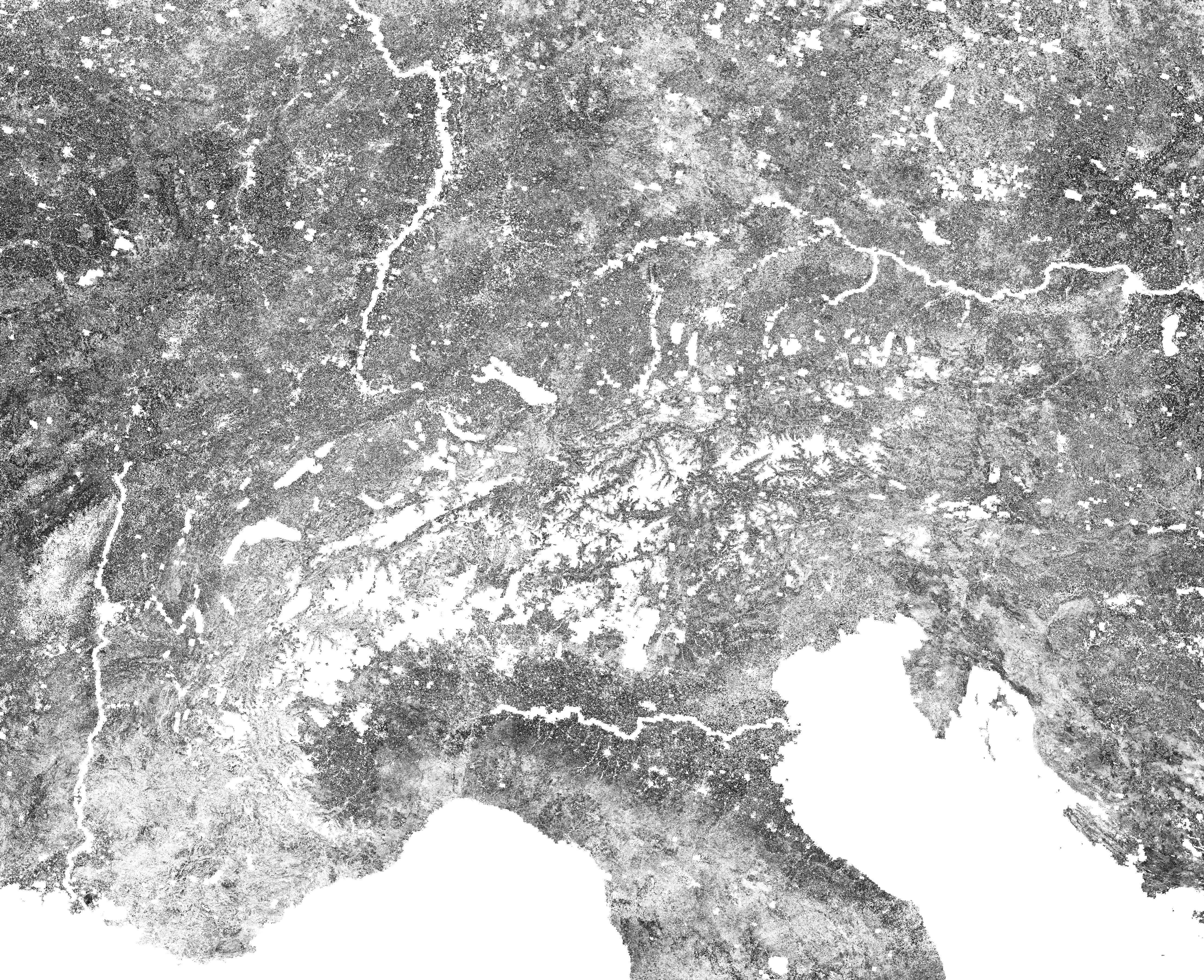
Vegetation Condition Index - 231 m 8 days
The Vegetation Condition Index (VCI) is based on the Normalized Difference Vegetation Index (NDVI) derived from MODIS satellite data. The NDVI is based on 8 day maximum value composite MOD09Q1 (v006) reflectance products. The spatial resolution is 231 m. The NDVI is masked to the highest quality standards using the provided quality layers. Missing pixel values in the time series are linearly interpolated. Non-vegetated areas are masked using the most recent Corine Land Cover product version for the according year. The final product is regridded to the LAEA Projection (EPSG:3035). The VCI is calculated using the formula VCIi = (NDVIi - NDVImin,i)/(NDVImax,i - NDVImin,i) * 100. The VCI expresses anomalies of the NDVI. The data is provided as 8 day measures. The time series is starting from 2001. The VCI values range from 0-100, whereas high values correspond to healthy vegetation and low values indicate stressed vegetation.
STAC
View
Jan. 1, 2001, 1 a.m.
None
None
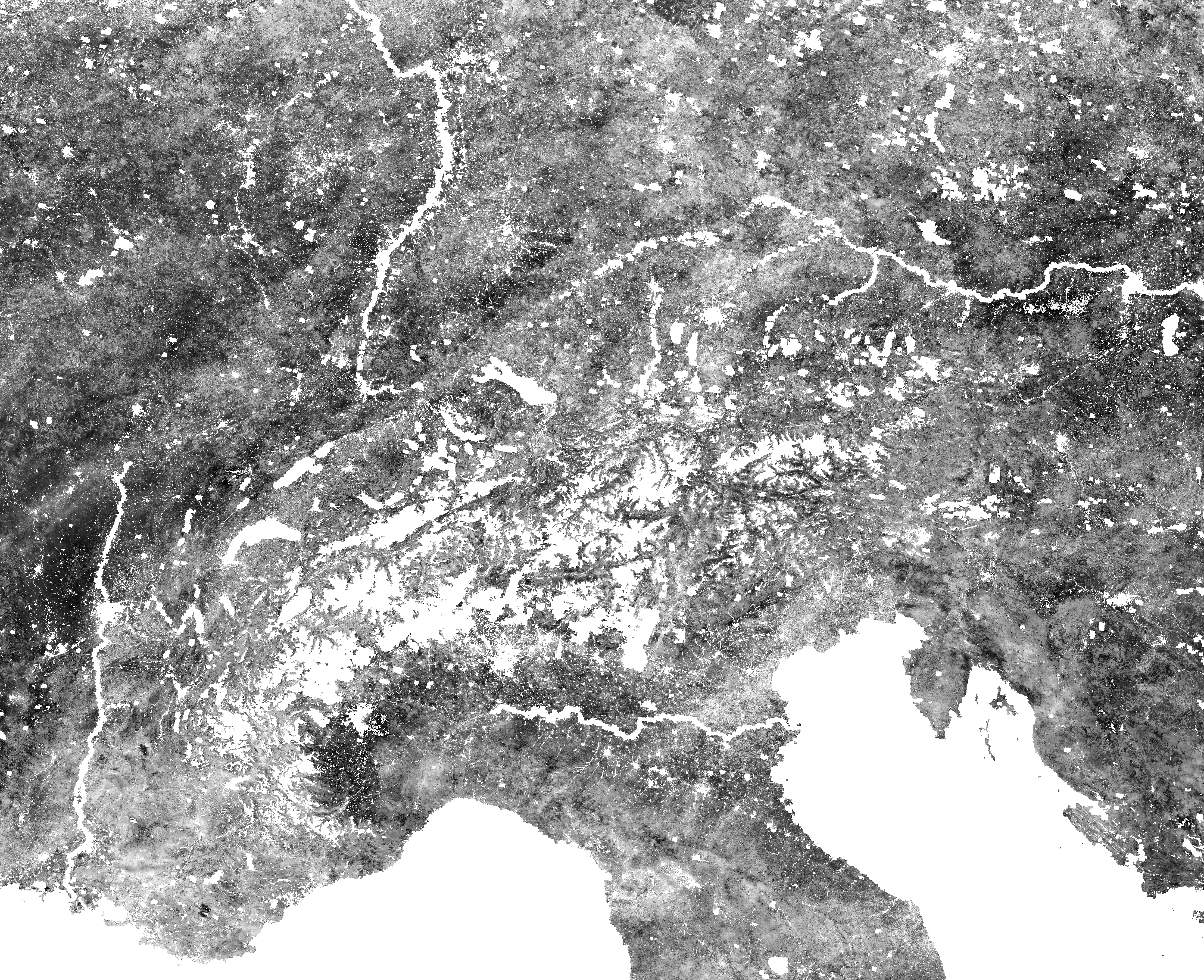
Vegetation Health Index - 231 m 8 days
The Vegetation Health Index (VHI) is based on a combination of products extracted from vegetation signals, namely the Normalized Difference Vegetation Index (NDVI) and the land surface temperature, both derived from MODIS satellite data. The NDVI is based on 8 day maximum value composite MOD09Q1 (v006) reflectance and the land surface temperature (LST) on 8 day MOD11A2 (v006) LST products. The spatial resolution is 231 m, therefore the original 1000 m resolution of the MOD11A2 LST is downscaled to 231 m of the MOD09Q1 reflectance. Both products are masked to the highest quality standards using the provided quality layers. Missing pixel values in the time series are linearly interpolated. Non-vegetated areas are masked using the most recent Corine Land Cover product version for the according year. The final product is regridded to the LAEA Projection (EPSG:3035). The VHI relies on a strong inverse correlation between NDVI and land surface temperature, since increasing land temperatures are assumed to act negatively on vegetation vigour and consequently to cause stress. The data is provided as 8 day measures. The time series is starting from 2001. The VHI values range from 0-100, whereas high values correspond to healthy vegetation and low values indicate stressed vegetation.
STAC
View
Jan. 1, 2001, 1 a.m.
None
None
Watt's Up? Synthetic Data for Buildings
This repository contains the challenge data and links to the participating teams' repositories for the Watt's Up? Hack for Energy Efficiency – Synthetic Data for Buildings hackathon, held at TU Wien on 22–23 February 2025. 🔗 Hackathon event page This hackathon was funded by the EU project MODERATE (grant No 101069834) and VSC/EuroCC.
Other
View
Weekly-aggregated irrigation product - Ebro basin
A 1 km experimental dataset of weekly-aggregated irrigation estimates retrieved through the SM-based inversion approach implemented with RT1 Sentinel-1 soil moisture and ERA5-Land rainfall and GLEAM 1 km potential evaporation
STAC
View
Jan. 1, 2016, 1 a.m.
Dec. 31, 2021, 1 a.m.
Dec. 31, 2021, 1 a.m.
Weekly-aggregated irrigation product - Po basin
A 1 km experimental dataset of weekly-aggregated irrigation estimates retrieved through the SM-based inversion approach implemented with RT1 Sentinel-1 soil moisture and ERA5-Land rainfall and GLEAM 1 km potential evaporation
STAC
View
Jan. 1, 2016, 1 a.m.
Dec. 31, 2021, 1 a.m.
Dec. 31, 2021, 1 a.m.
Wetlands_Dunes_Circeo_national_park
This collection is based on Sentinel-2 level 2A dataset acquired from both Sentinel-2 A and B satellites.
It covers a temporal range of 01-02-2021 to 30-09-2023, for every site all Sentinel scenes covering the area are included.
The collection includes all bands at a resolution of 10 meters. The bands are listed below.
B02
B03
B04
B05
B06
B07
B08
B8A
B09
B11
B12
SCL
The Level-2A data includes a Scene Classification, the algorithm allows the detection of clouds, snow and cloud shadows and generation of a classification map.
Cloud screening is applied to the data in order to retrieve accurate atmospheric and surface parameters during the atmospheric correction step.
The L2A SCL map can also be a valuable input for further processing steps or data analysis.
The collection covers all sites of the Hyperecos project. The following sites are included with the spatial extent mentioned.
Cireco {'west': 12.870775000000037, 'east': 13.103782000000024, 'south': 41.22186599400004, 'north': 41.41504699400008}
Orbetello {'west': 11.181888751927033,'east': 11.455397318265538, 'south': 42.372996996314896, 'north': 42.50311599528868}
Sciliar - Catinaccio {'west': 11.506713000000047, 'east': 11.667129000000045, 'south': 46.440615996000076, 'north': 46.54040999600005}
Castel Porziano {'west': 12.345466114000033, 'east': 12.451677663000055, 'south': 41.65575504100008, 'north': 41.78393419900004}
Monte Bondone {'west': 11.027602448000039, 'east': 11.044658587000072, 'south': 45.98801759300005, 'north': 46.01382867600006}
Bosco Fontana {'west': 10.73031770800003, 'east': 10.757708439000055, 'south': 45.192834764000054, 'north': 45.20899297600005}
Hunsrück-Hochwald {"west": 6.98720747225448, "east": 7.28904390300005, "north": 49.7943764377934, "south": 49.60530142600001}
STAC
View
May 5, 2021, 2 a.m.
Sept. 27, 2023, 2 a.m.
Sept. 27, 2023, 2 a.m.